library(ggplot2)

te_paper  <- "#f5f4ee"
te_ink    <- "#16241d"
te_body   <- "#2c3a31"
te_forest <- "#275139"
te_rust   <- "#b5534e"
te_gold   <- "#c9b458"
te_line   <- "#dad9ca"

theme_datasheet <- function() {
  theme_minimal(base_size = 12) +
    theme(plot.background  = element_rect(fill = te_paper, colour = NA),
          panel.background = element_rect(fill = te_paper, colour = NA),
          panel.grid.major = element_line(colour = te_line, linewidth = 0.3),
          panel.grid.minor = element_blank(),
          text             = element_text(colour = te_body),
          plot.title       = element_text(colour = te_ink, face = "bold"),
          plot.subtitle    = element_text(colour = te_body),
          axis.text        = element_text(colour = te_body))
}Extinction dates from sighting records
R
extinction
conservation
simulation
statistics
ecology tutorial
Dating extinctions from sighting records in R: the Solow test’s false alarm rate in closed form, and how often the linear estimation bound misses a decline.
A small orchid was collected in the same valley for a century. The herbarium sheets and the field notebooks between them give a list of dated sightings: several in most decades before the drainage schemes, a handful afterwards, then two isolated records some years apart, and nothing since, although botanists have walked the valley in most summers. The conservation question is whether the plant is gone, and if it is, when it went. The data for that question are not counts and not a population model. They are a column of dates.
Two methods answer it from the dates alone, and both are in routine use. Solow (1993) gave a test of whether a species is still extant, with a p value that depends only on the number of sightings and the date of the last one. Roberts and Solow (2003) gave optimal linear estimation, which fits the spacing of the last few sightings and returns an estimated extinction date with an upper confidence bound; Roberts and Solow applied it to the dodo. Boakes, Rout and Collen (2015) compared these and several related methods, and McInerny and colleagues (2006) built a method around the sighting rate rather than the date of the last sighting.
This is the backward problem, and the blog so far has only worked the forward one. Mean time to extinction, exactly starts from a birth-death model and computes how long a population lasts; its central section shows persistence time growing exponentially with carrying capacity, and no sighting ever appears in it. Population viability analysis and extinction risk starts from a series of counts and projects the chance of falling below a threshold. Decline estimates and Red List criterion A turns a monitored index into a reduction and a category. Records as a test for trend counts record values in a series of measurements, which is a different object from the times of discrete events. Here the population is never observed directly, and the only evidence is when somebody saw it.
The decision the methods feed is real but it is not theirs to make. The IUCN Red List can flag a Critically Endangered species as Possibly Extinct, and that flag is an assessor’s judgement that weighs survey effort, threats and the record together. A p value or an upper bound from a sighting record is one line of evidence in such an assessment, not a rule that assigns the tag, and nothing below should be read as saying otherwise.
The post does three things. It derives the false extinction rate of the Solow test when a still extant species has a declining sighting rate, in closed form, and checks the formula by simulation. It implements optimal linear estimation exactly as Roberts and Solow define it and checks its upper bound on a species that vanishes all at once. Then it runs the estimator on a population that dwindles animal by animal, and measures how often the upper bound on the extinction date lies after the true date.
The Solow test has a closed form false alarm rate
Solow’s test treats the observation window as running from zero to T, with n sightings at times up to the last one, t_n. Under the null hypothesis the species is extant throughout and sightings arrive as a Poisson process with a constant rate, so given n the sighting times are independent and uniform on the window. The largest of n uniform times falls below x with probability (x / T) to the power n, and that gives the p value directly: p = (t_n / T)^n. A small p means the last sighting came suspiciously early, and the species is declared extinct.
The same argument gives the false alarm rate when the rate is not constant. Suppose the species is still there at T but is being seen less and less, with sighting times that, given n, are independent with a distribution function F on the window. The test rejects when (t_n / T)^n is below alpha, which is when t_n is below T alpha^(1/n), and the maximum of n independent times is below that value with probability F(T alpha(1/n))n. Averaging over the Poisson distribution of n, and leaving out the records with no sighting at all, gives the exact rate. For a constant rate F is uniform and every term equals alpha, which is the calibration check.
The design below fixes the window at fifty years, the expected number of sightings at twenty, and lets the sighting rate decline exponentially so that it ends one, two, five or ten times lower than it started. These constants were set before anything ran.
t_win   <- 50
lam_tot <- 20
alpha   <- 0.05
dec_fac <- c(1, 2, 5, 10)

cdf_decl <- function(x, r_decl) {
  if (r_decl == 0) return(x / t_win)
  (1 - exp(-r_decl * x)) / (1 - exp(-r_decl * t_win))
}
solow_exact <- function(d_fac) {
  r_decl <- log(d_fac) / t_win
  n_seq  <- 1:400
  sum(dpois(n_seq, lam_tot) * cdf_decl(t_win * alpha^(1 / n_seq), r_decl)^n_seq) /
    (1 - dpois(0, lam_tot))
}
exact_rate <- vapply(dec_fac, solow_exact, 0)
t_cut20    <- t_win * alpha^(1 / lam_tot)
n_solow <- 10000
set.seed(1993)
solow_sim <- vapply(dec_fac, function(d_fac) {
r_decl <- log(d_fac) / t_win
n_sight <- rpois(n_solow, lam_tot)
n_sight <- n_sight[n_sight > 0]
run_id <- rep(seq_along(n_sight), n_sight)
u_draw <- runif(length(run_id))
t_draw <- if (d_fac == 1) t_win * u_draw else
-log(1 - u_draw * (1 - exp(-r_decl * t_win))) / r_decl
t_last <- tapply(t_draw, run_id, max)
mean((t_last / t_win)^n_sight < alpha)
}, 0)
solow_se <- sqrt(solow_sim * (1 - solow_sim) / n_solow)
solow_z <- max(abs(solow_sim - exact_rate) / solow_se)
p_zero <- dpois(0, lam_tot)With a constant rate the exact false extinction rate is 0.0500, which is alpha, as it must be. When the rate halves over the window it is 0.118; with a fivefold decline 0.272; with a tenfold decline 0.422. In every one of these records the species is alive at the end of the window.
The simulation draws every sighting time, not only the last, from 10000 records per decline factor. The simulated rates are 0.0528, 0.122, 0.271 and 0.425, and the largest distance from the formula is 1.4 Monte Carlo standard errors. Records with no sighting (probability 2.06e-09 at this design) are dropped in both.
So the first result needs no simulation at all. A declining sighting rate is the null hypothesis being false in the direction that mimics extinction, and the test responds the way any test does to a false null. The formula also shows what drives the inflation: the distribution function F evaluated at T alpha^(1/n), which for a record of twenty sightings is year 43.0 of 50, so the rate is set by the share of the sighting rate that falls in the last 7 years of the window.
d_grid  <- seq(1, 10, by = 0.1)
curve_df <- data.frame(d_fac = d_grid, rate = vapply(d_grid, solow_exact, 0))
sim_df   <- data.frame(d_fac = dec_fac, rate = solow_sim,
                       lo = solow_sim - 2 * solow_se, hi = solow_sim + 2 * solow_se)

ggplot(curve_df, aes(d_fac, rate)) +
  geom_hline(yintercept = alpha, linetype = "dashed", colour = te_body, linewidth = 0.6) +
  geom_line(colour = te_forest, linewidth = 1) +
  geom_errorbar(data = sim_df, aes(ymin = lo, ymax = hi), width = 0.15,
                colour = te_rust, linewidth = 0.6) +
  geom_point(data = sim_df, colour = te_rust, size = 2.6) +
  scale_x_continuous(breaks = c(1, 2, 4, 6, 8, 10)) +
  scale_y_continuous(limits = c(0, NA)) +
  labs(x = "decline in sighting rate over the window (start rate / end rate)",
       y = "probability of declaring extinct",
       title = "An extant, fading species fails the test",
       subtitle = "line: exact formula; points: simulation, two standard errors; dashed: alpha") +
  theme_datasheet()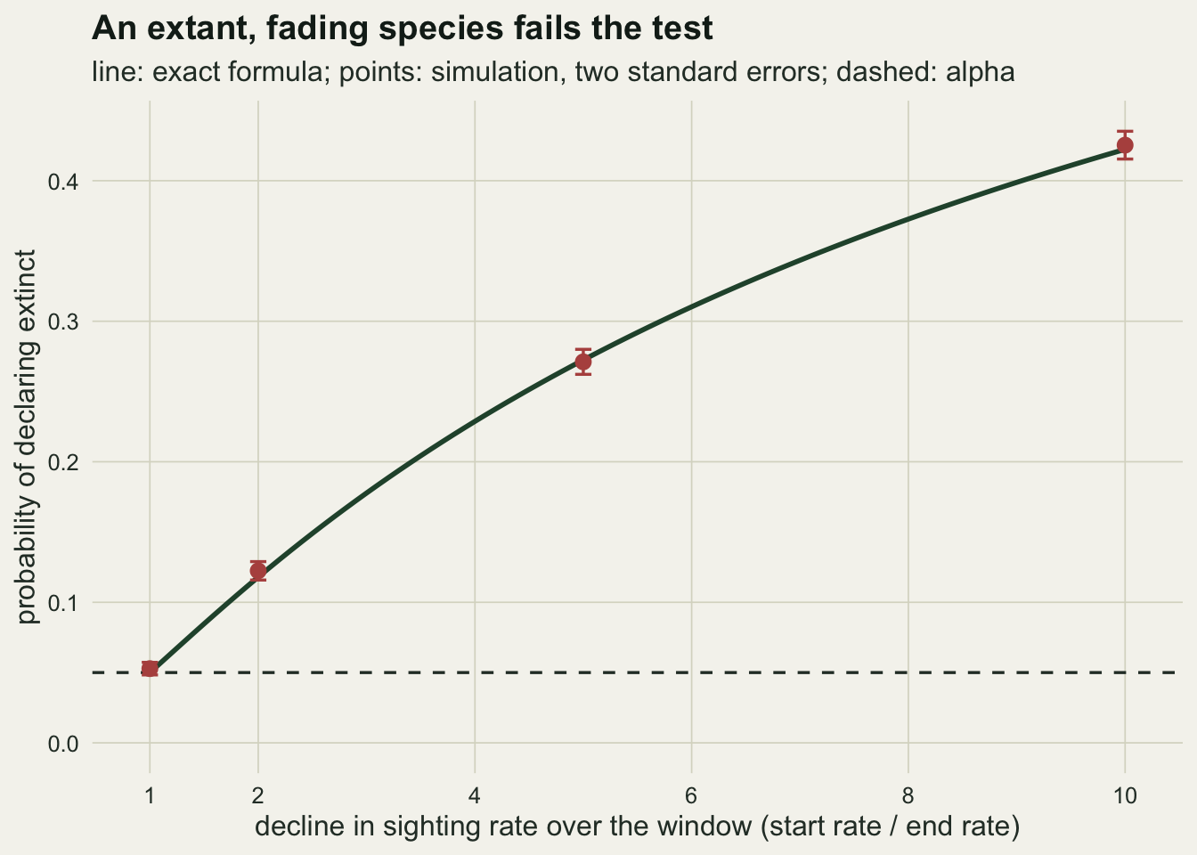
Optimal linear estimation, as defined
Roberts and Solow start from a result in extreme value theory: the few most recent sightings of a species that has gone extinct behave like the largest values of a sample from a distribution with a finite endpoint, and near that endpoint the joint distribution of the top k values has a Weibull form with a shape parameter v, whatever the process was earlier. The extinction date is the endpoint. With the sightings ordered from the most recent, t_1 > t_2 > … > t_k, the method has four steps, and the code below follows them line by line.
The shape is estimated as v = (1 / (k - 1)) times the sum over i from 1 to k - 2 of log((t_1 - t_k) / (t_1 - t_(i+1))). A k by k matrix Lambda is filled with Gamma(2v + i) Gamma(v + j) / (Gamma(v + i) Gamma(j)) for j no larger than i, and made symmetric. The weights are a = (e’ Lambda^-1 e)^-1 Lambda^-1 e, with e a column of ones, and the point estimate of the extinction date is the weighted sum of the t_i. The upper bound of a one sided confidence interval at level 1 - alpha is t_1 + (t_1 - t_k) / (S - 1), with S = (-log(alpha) / k)^(-v).
That definition was checked against the formulae as reproduced in the OLE.fun source of the archived sExtinct package, which computes the same v, the same Lambda and the same bound. One difference matters: that function reports a two sided interval and uses alpha / 2 in S. The bound here is one sided at alpha = 0.05, a 95 per cent upper bound, which is the quantity a reader wants when the question is how late the species could have survived.
ole_fit <- function(t_sight, k_last, level_alpha = 0.05) {
  t_ord <- sort(t_sight, decreasing = TRUE)[seq_len(k_last)]
  v_hat <- sum(log((t_ord[1] - t_ord[k_last]) /
                   (t_ord[1] - t_ord[2:(k_last - 1)]))) / (k_last - 1)
  i_max <- outer(seq_len(k_last), seq_len(k_last), pmax)
  j_min <- outer(seq_len(k_last), seq_len(k_last), pmin)
  lam_mat <- exp(lgamma(2 * v_hat + i_max) + lgamma(v_hat + j_min) -
                 lgamma(v_hat + i_max) - lgamma(j_min))
  w_raw <- solve(lam_mat, rep(1, k_last))
  w_ole <- w_raw / sum(w_raw)
  s_up  <- (-log(level_alpha) / k_last)^(-v_hat)
  c(estimate = sum(w_ole * t_ord),
    upper    = t_ord[1] + (t_ord[1] - t_ord[k_last]) / (s_up - 1),
    v_hat    = v_hat)
}
k_grid <- c(5, 10, 20)
k_keep <- max(k_grid)
The check is the case the method is built for. A population of 200 animals, each seen 0.05 times a year, is present at full size for sixty years and then disappears in one step, so sightings are a constant-rate Poisson process that stops dead at the extinction date. For a constant rate stopping at an endpoint the Weibull shape is exactly one, and the coverage of the upper bound should sit near 0.95.
n0_pop   <- 200
te_abr   <- 60
c_low    <- 0.05
c_high   <- 0.5
n_run    <- 2000

eval_ole <- function(run_list, k_vals = k_grid) {
  do.call(rbind, lapply(k_vals, function(k_last) {
    out <- t(vapply(run_list, function(rr) {
      if (length(rr$t_last) < k_last) return(rep(NA_real_, 5))
      c(ole_fit(rr$t_last, k_last), rr$t_ext, rr$t_last[1])
    }, numeric(5)))
    ok_run <- !is.na(out[, 1])
    cov_hat <- mean(out[ok_run, 2] >= out[ok_run, 4])
    data.frame(k = k_last, cover = cov_hat,
               cover_se = sqrt(cov_hat * (1 - cov_hat) / sum(ok_run)),
               n_ok = sum(ok_run),
               width = median(out[ok_run, 2] - out[ok_run, 5]),
               lag_true = median(out[ok_run, 4] - out[ok_run, 5]),
               bias = median(out[ok_run, 1] - out[ok_run, 4]),
               v_med = median(out[ok_run, 3]))
  }))
}

set.seed(2003)
abr_runs <- lapply(seq_len(n_run), function(i) {
  n_s <- rpois(1, n0_pop * c_low * te_abr)
  list(t_last = sort(runif(n_s, 0, te_abr), decreasing = TRUE)[seq_len(k_keep)],
       t_ext = te_abr)
})
abr_tab <- eval_ole(abr_runs)
abr_mcse <- max(abr_tab$cover_se)
abr_z20  <- (0.95 - abr_tab$cover[3]) / abr_tab$cover_se[3]
Over 2000 records the upper bound covers the true date in 0.983 of runs with k = 5, 0.956 with k = 10 and 0.940 with k = 20, with Monte Carlo standard errors up to 0.005. The median estimated shape at k = 10 is 0.85 against the true value of one. The bound is conservative for small k, where the shape rests on very few gaps, and at k = 20 it sits 1.9 Monte Carlo standard errors below nominal. That small shortfall is part of the method, and it is the reference against which the dwindling populations are read.
A population that dwindles
A real extinction is rarely a step. The simulation below follows a closed population of 200 animals with annual survival of 0.93 or 0.97 and no recruitment, so numbers fall geometrically on average and the last few animals linger for a stochastic stretch of years. Each year every live animal can be seen, and the number of sightings is Poisson with mean c times the number alive, at c = 0.05 or c = 0.5 sightings per animal per year; each sighting is placed at a uniform time within its year. The true extinction date is the end of the last year in which any animal was alive. Sightings in that year are spread over the whole year, so the sighting process stops at exactly that date, as it stops at year 60 in the abrupt control. The design and the 2000 runs per cell were fixed before running.
sim_dwindle <- function(n_run, s_ann, c_rate, n_start = n0_pop) {
  alive <- rep(n_start, n_run)
  n_list <- list()
  while (any(alive > 0)) {
    n_list[[length(n_list) + 1]] <- alive
    alive <- rbinom(n_run, alive, s_ann)
  }
  n_mat  <- do.call(cbind, n_list)
  s_mat  <- matrix(rpois(length(n_mat), c_rate * n_mat), n_run)
  t_ext  <- rowSums(n_mat > 0)
  path_1 <- list(alive = n_mat[1, seq_len(t_ext[1])],
                 counts = s_mat[1, seq_len(t_ext[1])])
  runs_out <- lapply(seq_len(n_run), function(i) {
    cnt_i  <- s_mat[i, seq_len(t_ext[i])]
    rev_cs <- rev(cumsum(rev(cnt_i)))
    yr_use <- which(rev_cs - cnt_i < k_keep)
    t_i    <- rep(yr_use - 1, cnt_i[yr_use]) + runif(sum(cnt_i[yr_use]))
    if (i == 1) {
      path_1$t_used <<- t_i
      path_1$first_used <<- min(yr_use)
    }
    list(t_last = sort(t_i, decreasing = TRUE)[seq_len(min(k_keep, length(t_i)))],
         t_ext = t_ext[i], n_total = sum(cnt_i))
  })
  attr(runs_out, "path") <- path_1
  runs_out
}

cells <- data.frame(s_ann = c(0.93, 0.97, 0.93, 0.97),
                    c_rate = c(c_low, c_low, c_high, c_high))
set.seed(2015)
cell_runs <- lapply(seq_len(nrow(cells)), function(j)
  sim_dwindle(n_run, cells$s_ann[j], cells$c_rate[j]))
cell_tab <- do.call(rbind, lapply(seq_len(nrow(cells)), function(j)
  cbind(cells[j, ], eval_ole(cell_runs[[j]]), row.names = NULL)))
te_med   <- vapply(cell_runs, function(rr) median(vapply(rr, `[[`, 0, "t_ext")), 0)
min_ok   <- min(cell_tab$n_ok)
pick <- function(s_val, c_val, k_val, col) {
cell_tab[cell_tab$s_ann == s_val & cell_tab$c_rate == c_val & cell_tab$k == k_val, col]
}
cov_93lo <- vapply(k_grid, function(k) pick(0.93, c_low, k, "cover"), 0)
cov_97lo <- vapply(k_grid, function(k) pick(0.97, c_low, k, "cover"), 0)
cov_93hi <- vapply(k_grid, function(k) pick(0.93, c_high, k, "cover"), 0)
cov_97hi <- vapply(k_grid, function(k) pick(0.97, c_high, k, "cover"), 0)
se_worst <- max(cell_tab$cover_se)
lag_93lo <- pick(0.93, c_low, 10, "lag_true")
lag_93hi <- pick(0.93, c_high, 10, "lag_true")
wid_93lo <- vapply(k_grid, function(k) pick(0.93, c_low, k, "width"), 0)
v_93lo <- pick(0.93, c_low, 10, "v_med")
bias_all <- cell_tab$bias
drop_10_20 <- cov_93lo[2] - cov_93lo[3]
k10_all <- c(abr_tab$cover[2], cell_tab$cover[cell_tab$k == 10])
k20_all <- c(abr_tab$cover[3], cell_tab$cover[cell_tab$k == 20])
n_k_down <- sum(k20_all < k10_all)
n_k_cells <- length(k10_all)
lag_97lo <- pick(0.97, c_low, 10, "lag_true")
wid_97lo <- pick(0.97, c_low, 10, "width")
miss_10 <- 1 - cov_93lo[2]
miss_ratio <- miss_10 / 0.05
gap_hi_abr <- (abr_tab$cover[2] - cov_93hi[2]) /
sqrt(abr_tab$cover_se[2]^2 + pick(0.93, c_high, 10, "cover_se")^2)
v_97lo <- pick(0.97, c_low, 10, "v_med")
alive_at_k <- 10 * (1 - 0.93) / c_lowrun_mat <- function(run_list) {
t(vapply(run_list, function(rr) {
f10 <- ole_fit(rr$t_last, 10)
f20 <- ole_fit(rr$t_last, 20)
c(up10 = f10[["upper"]], up20 = f20[["upper"]], v10 = f10[["v_hat"]],
t_ext = rr$t_ext, t_1 = rr$t_last[1], span10 = rr$t_last[1] - rr$t_last[10])
}, numeric(6)))
}
scen_mats <- lapply(c(list(abr_runs), cell_runs), run_mat)
pair_z <- vapply(scen_mats, function(m) {
d_cov <- (m[, "up10"] >= m[, "t_ext"]) - (m[, "up20"] >= m[, "t_ext"])
mean(d_cov) / (sd(d_cov) / sqrt(nrow(m)))
}, 0)
n_k_clear <- sum(pair_z > 2)
z_93lo <- pair_z[2]
z_min <- min(pair_z)
span_93lo <- median(scen_mats[[2]][, "span10"])
span_97lo <- median(scen_mats[[3]][, "span10"])
v_iqr_93 <- quantile(scen_mats[[2]][, "v10"], c(0.25, 0.75))
v_iqr_97 <- quantile(scen_mats[[3]][, "v10"], c(0.25, 0.75))In every run the population went extinct and every record had at least 20 sightings (the smallest usable count across cells is 2000 of 2000). The median extinction year is 78 at survival 0.93 and 186 at 0.97.
ex_run  <- cell_runs[[1]][[1]]
ex_path <- attr(cell_runs[[1]], "path")
ex_fit  <- ole_fit(ex_run$t_last, 10)
pop_df  <- data.frame(year = seq_along(ex_path$alive) - 1, alive = ex_path$alive)
early_yr  <- seq_len(ex_path$first_used - 1)
set.seed(11)
early_t   <- rep(early_yr - 1, ex_path$counts[early_yr]) +
  runif(sum(ex_path$counts[early_yr]))
all_sight <- c(early_t, ex_path$t_used)
sight_df  <- data.frame(t_s = all_sight,
                        used = all_sight >= ex_run$t_last[10])
ex_lines  <- data.frame(x = c(ex_run$t_ext, ex_fit[["upper"]]),
                        what = c("true extinction", "upper bound, k = 10"))
ex_nsight <- length(all_sight)

ggplot(pop_df, aes(year, alive)) +
  geom_step(colour = te_forest, linewidth = 0.8) +
  geom_rug(data = sight_df, aes(x = t_s, colour = used), inherit.aes = FALSE,
           sides = "b", length = grid::unit(0.06, "npc"), linewidth = 0.5) +
  geom_vline(data = ex_lines, aes(xintercept = x, linetype = what),
             colour = te_rust, linewidth = 0.8) +
  scale_colour_manual(values = c(`FALSE` = te_body, `TRUE` = te_gold),
                      labels = c("earlier sighting", "last ten sightings"), name = NULL) +
  scale_linetype_manual(values = c("dashed", "solid"), name = NULL) +
  labs(x = "year", y = "animals alive",
       title = "One record from a dwindling population",
       subtitle = "ticks on the axis: sighting times") +
  theme_datasheet() +
  theme(legend.position = "bottom")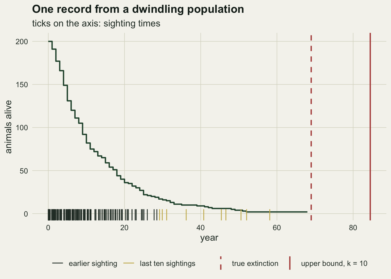
The figure shows the first simulated record in the harshest cell, not a chosen one. The population leaves 130 sightings in total, dense while the animals are numerous and thinning to isolated ticks as the last few survive. The last animal is gone by year 69; the ten most recent sightings put the upper bound at 84.5, so in this record the bound holds, 26.4 years after the last sighting at 58.1. The question is how often it holds.
Across the four dwindling cells the coverage table reads as follows. At survival 0.93 and 0.05 sightings per animal per year, coverage is 0.921, 0.843 and 0.824 for k = 5, 10 and 20. At survival 0.97 and the same sighting rate it is 0.944, 0.882 and 0.864. With ten times the sighting rate it returns to 0.965, 0.928 and 0.924 at survival 0.93, and 0.977, 0.945 and 0.935 at 0.97. No Monte Carlo standard error in the table exceeds 0.0085.
cov_df <- rbind(
  data.frame(k = abr_tab$k, cover = abr_tab$cover, se = abr_tab$cover_se,
             scen = "abrupt, 0.05 per animal-year"),
  data.frame(k = cell_tab$k, cover = cell_tab$cover, se = cell_tab$cover_se,
             scen = sprintf("survival %.2f, %.2f per animal-year",
                            cell_tab$s_ann, cell_tab$c_rate)))
ggplot(cov_df, aes(k, cover, colour = scen)) +
  geom_hline(yintercept = 0.95, linetype = "dashed", colour = te_body, linewidth = 0.6) +
  geom_line(linewidth = 0.9, position = position_dodge(width = 0.8)) +
  geom_errorbar(aes(ymin = cover - 2 * se, ymax = cover + 2 * se), width = 0.6,
                linewidth = 0.5, position = position_dodge(width = 0.8)) +
  geom_point(size = 2.3, position = position_dodge(width = 0.8)) +
  scale_x_continuous(breaks = k_grid) +
  scale_colour_manual(values = c("#7a8f80", te_rust, te_forest, te_gold, "#5f7fa6"), name = NULL) +
  guides(colour = guide_legend(ncol = 2)) +
  labs(x = "last sightings used (k)", y = "coverage of the upper bound",
       title = "Sparse tails break the bound",
       subtitle = "bars: two Monte Carlo standard errors; dashed: nominal 0.95") +
  theme_datasheet() +
  theme(legend.position = "bottom")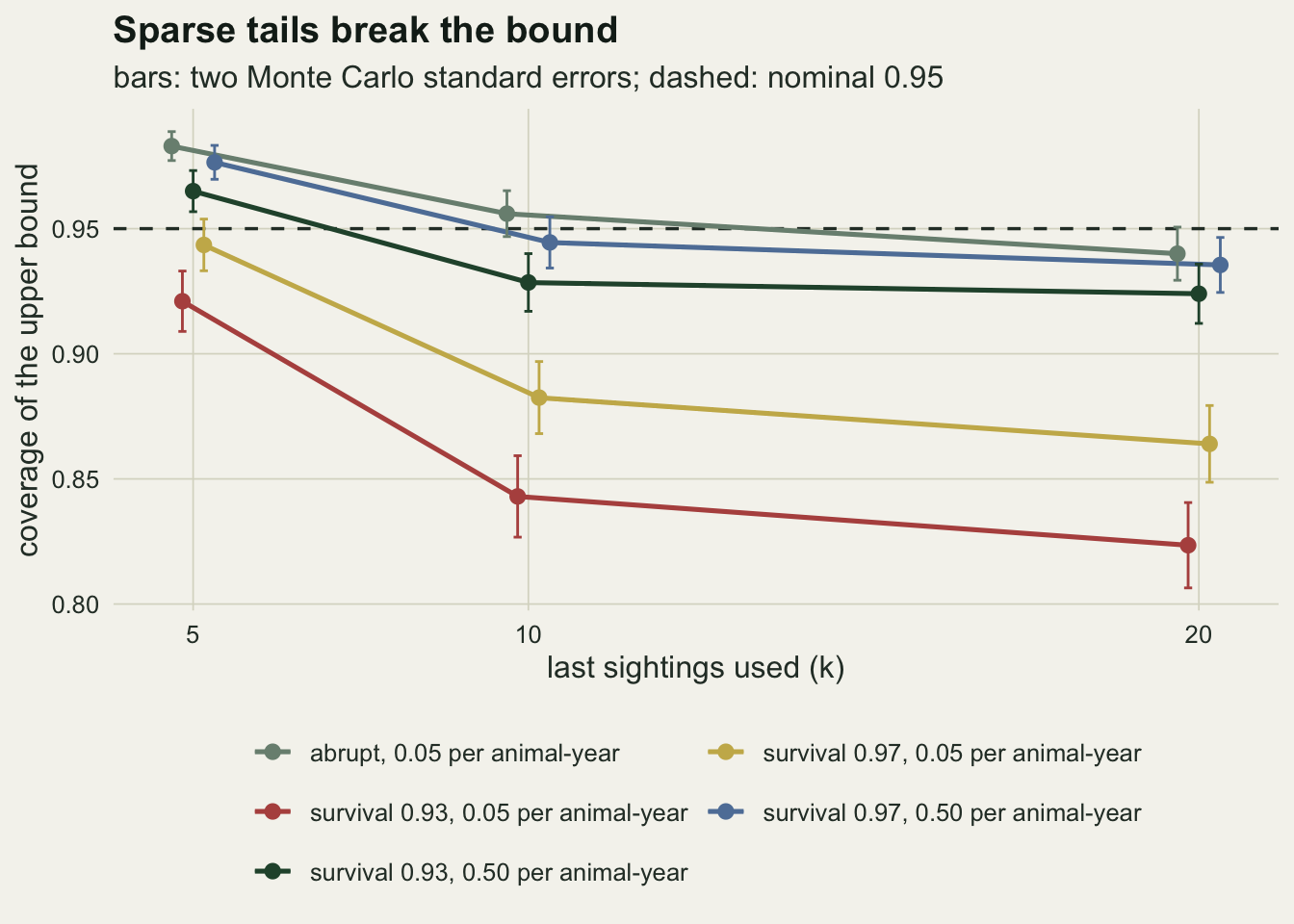
The abrupt control stays near nominal. The failure is the dwindling population at the low sighting rate: at k = 10 the bound falls before the true extinction date in 0.157 of records, 3.1 times the five per cent the interval promises. Using more of the record does not help. Going from ten to twenty sightings lowers coverage by 0.019, which is 4.2 standard errors of the paired difference (both bounds are computed on the same runs). Across the 5 scenarios in the figure, coverage at k = 20 is lower than at k = 10 in 5, and by more than two paired standard errors in 4; the weakest of the 5 is 1.3 standard errors. Five sightings cover better, 0.921, but only because the bound is then very wide: its median distance beyond the last sighting is 76 years at k = 5, against 38 at k = 10 and 32 at k = 20.
Raising the sighting rate tenfold brings coverage at k = 10 back to 0.928 at survival 0.93. That is most of the way to the abrupt control’s 0.956, but not all of it: the remaining gap is 3.7 standard errors. At the low sighting rate the slower decline covers better than the faster one, 0.882 against 0.843 at k = 10, although its last animals go unseen for longer (a median of 12.4 years against 9.8): its last ten sightings are also more spread out (they span a median of 54.6 years against 28.9), and the median bound lies 59 years beyond the last sighting against 38. What decides a miss is the silent stretch measured against the spacing of the sightings before it, and the next section measures that.
The point estimate behaves less consistently. Its median error across the 12 combinations of dwindling cell and k runs from -0.6 to +4.8 years, taking both signs, so no general statement about early or late estimates can be made from this design, and none is made here.
Why more sightings do not repair it
Optimal linear estimation does allow the sighting rate to change towards the end: the shape v absorbs a rate that falls as a power of the time left. What it cannot see is a stretch with no sightings at all. At 0.05 sightings per animal per year a single surviving animal is seen, on average, once in 20 years, and the last one or two animals of a dwindling population can outlive their final sighting by a decade. The bound is built from the spacing of the last k sightings, and they were made while more animals were alive. A rough expectation makes the point: ten sightings at this rate take 200 animal-years, and a geometric decline at survival 0.93 accumulates that many animal-years after the population passes about 14 animals, so the tenth-last sighting typically falls when that many were still alive and sightings came close together. Adding sightings reaches further back into the dense part of the record, which tightens the spacing and pulls the bound in; it does nothing to the silent tail.
low_runs <- cell_runs[[1]]
gap_df <- do.call(rbind, lapply(low_runs, function(rr) {
  fit <- ole_fit(rr$t_last, 10)
  data.frame(lag_true = rr$t_ext - rr$t_last[1],
             lag_bound = fit[["upper"]] - rr$t_last[1])
}))
gap_df$miss <- gap_df$lag_bound < gap_df$lag_true
miss_share  <- mean(gap_df$miss)
lag_q90     <- quantile(gap_df$lag_true, 0.9)
lag_miss_med <- median(gap_df$lag_true[gap_df$miss])
lag_hit_med  <- median(gap_df$lag_true[!gap_df$miss])
last_one <- vapply(low_runs, function(rr) rr$t_ext - rr$t_last[1], 0)
gap_df$span10 <- scen_mats[[2]][, "span10"]
auc_miss <- function(score, is_miss) {
  rk <- rank(score)
  (sum(rk[is_miss]) - sum(is_miss) * (sum(is_miss) + 1) / 2) /
    (sum(is_miss) * sum(!is_miss))
}
auc_lag   <- auc_miss(gap_df$lag_true, gap_df$miss)
auc_ratio <- auc_miss(gap_df$lag_true / gap_df$span10, gap_df$miss)
rho_span <- cor(gap_df$lag_true, gap_df$span10, method = "spearman")ggplot(gap_df, aes(lag_true, lag_bound, colour = miss)) +
geom_abline(slope = 1, intercept = 0, colour = te_ink, linewidth = 0.6) +
geom_point(size = 1, alpha = 0.55) +
scale_x_log10() + scale_y_log10() +
scale_colour_manual(values = c(`FALSE` = te_forest, `TRUE` = te_rust),
labels = c("bound after true date", "bound before true date"), name = NULL) +
labs(x = "years from last sighting to extinction (log scale)",
y = "years from last sighting to upper bound (log scale)",
title = "The misses are the long silent tails",
subtitle = "one point per simulated record; line: bound equals true date") +
theme_datasheet() +
theme(legend.position = "bottom")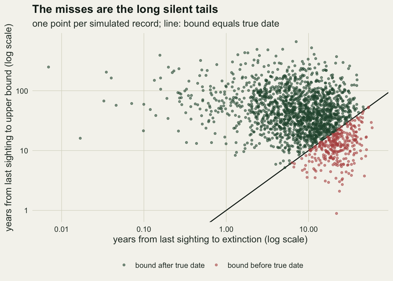
In this cell the median time from the last sighting to extinction is 9.8 years, and one record in ten waits more than 25 years. The bound misses in 0.157 of records at k = 10, and the misses are not scattered across the plot: their median silent stretch is 22.3 years, against 8.0 years in the records the bound covers. At the tenfold sighting rate the median silent stretch is 1.3 years. The misses are the records whose silent tail is long relative to the spacing of the sightings that precede it. Ranked by the silent stretch alone, a missed record outranks a covered one with probability 0.892; ranked by the silent stretch divided by the span of the last ten sightings, with probability 0.946. The spacing the sightings do carry points the wrong way: the rank correlation between the silent stretch and that span is -0.36, so longer silent tails go with tighter last spacings, and a tighter spacing pulls the bound in.
What to report
For the Solow test, report the p value together with what is known about how the sighting rate changed over the window. The exact false extinction rate under any assumed decline is the formula in the first section, a one line sum in R, and quoting it for a plausible decline tells a reader how much of a small p value could be detectability falling rather than the species going. A tenfold decline with twenty expected sightings turned a five per cent test into one that declared a living species extinct in 0.42 of records.
For optimal linear estimation, report k, the one sided level of the bound and the span of the k sightings used, and show the bound for more than one k. Do not treat a larger k as the safer choice; in the dwindling cells it narrowed the interval and lowered coverage together.
Report the number of years since the last sighting next to whatever is known about the sighting rate per surviving individual. When that rate is low, the silent stretch at the end of a decline is long, and a bound computed from the last sightings can be expected to fall short of the true date more often than its nominal level; at the lowest rate simulated here it did so in one record in 6.4 at k = 10.
Name the decision correctly. A p value or a bound is evidence that an assessor can weigh when considering the Possibly Extinct tag on the Red List, alongside the survey effort that failed to find the species and the state of its threats. It does not assign that tag, and a record that passes either method with a comfortable margin can still belong to a species that is gone.
Honest limits
The population model is deliberately plain: a closed population with no recruitment, a fixed annual survival and independent deaths. Real declines include failed recruitment, habitat loss that removes animals in blocks, and Allee effects that speed up the final years. The shape of the tail is what decides coverage, and it is not identifiable from the last sightings themselves: the median estimated shape at k = 10 is 0.47 at survival 0.93 (interquartile range 0.33 to 0.66) and 0.54 at 0.97 (0.38 to 0.74), two declines whose median extinction years are 78 and 186, so the two interquartile ranges overlap from 0.38 to 0.66 and the fitted v cannot tell a user which of these two declines produced a record.
Sightings here arrive as a Poisson process with a constant rate per animal and constant effort. Real records mix collections, casual reports and dedicated surveys whose effort changes over decades, and some late sightings are wrong. Both problems are outside this simulation. McInerny and colleagues build the sighting rate into their method, and Boakes, Rout and Collen discuss how the methods compare when the record departs from their assumptions.
The population is counted once a year, and an animal alive at the start of its last year is seen at a constant rate until the end of that year. In a real decline the last animal dies partway through a year and its sightings stop there, which removes late sightings as well as moving the date. The check below gives every animal that dies in a year a uniform death time, stops its sightings at that time, and measures coverage against the death of the last animal, at survival 0.93 and both sighting rates.
sim_cont <- function(n_run_c, s_ann, c_rate, n_start = n0_pop) {
  lapply(seq_len(n_run_c), function(i) {
    n_now <- n_start; yr <- 0; t_s <- numeric(0)
    while (n_now > 0) {
      n_next <- rbinom(1, n_now, s_ann)
      u_die  <- runif(n_now - n_next)
      s_die  <- rpois(length(u_die), c_rate * u_die)
      t_s <- c(t_s, yr + runif(rpois(1, c_rate * n_next)),
               yr + runif(sum(s_die)) * rep(u_die, s_die))
      if (n_next == 0) t_death <- yr + max(u_die)
      n_now <- n_next; yr <- yr + 1
    }
    list(t_last = sort(t_s, decreasing = TRUE)[seq_len(min(k_keep, length(t_s)))],
         t_ext = t_death)
  })
}
set.seed(2016)
cont_tab <- vapply(c(c_low, c_high), function(c_val) {
  rr <- sim_cont(n_run, 0.93, c_val)
  ok <- vapply(rr, function(r) length(r$t_last) >= 10, TRUE)
  up <- vapply(rr[ok], function(r) ole_fit(r$t_last, 10)[["upper"]], 0)
  c(cover = mean(up >= vapply(rr[ok], `[[`, 0, "t_ext")), n_ok = sum(ok))
}, numeric(2))
cont_se  <- sqrt(cont_tab["cover", ] * (1 - cont_tab["cover", ]) / cont_tab["n_ok", ])
gap_cont <- (abr_tab$cover[2] - cont_tab["cover", 2]) /
  sqrt(abr_tab$cover_se[2]^2 + cont_se[2]^2)
With continuous deaths, coverage at k = 10 is 0.822 at the low sighting rate and 0.934 at the tenfold rate (Monte Carlo standard errors up to 0.0086, from 2000 usable records per cell), against 0.843 and 0.928 in the yearly model. The high rate still falls 3.0 standard errors short of the abrupt control, so neither conclusion rests on counting the population once a year.
The Solow numbers are for an exponential decline in rate with twenty expected sightings over fifty years. The formula holds for any sighting time distribution, but the particular rates quoted do not transfer to other windows or record sizes without rerunning the sum.
Only two methods are measured. Boakes, Rout and Collen compared several related methods, and none of the others is tested here. The coverage rates of the four dwindling cells carry Monte Carlo standard errors up to 0.0085 from 2000 runs per cell.
References
Solow AR 1993 Ecology 74(3):962-964 (10.2307/1940821)
Roberts DL, Solow AR 2003 Nature 426(6964):245 (10.1038/426245a)
McInerny GJ, Roberts DL, Davy AJ, Cribb PJ 2006 Conservation Biology 20(2):562-567 (10.1111/j.1523-1739.2006.00377.x)
Boakes EH, Rout TM, Collen B 2015 Methods in Ecology and Evolution 6(6):678-687 (10.1111/2041-210X.12365)