library(ggplot2)

te_paper  <- "#f5f4ee"
te_ink    <- "#16241d"
te_body   <- "#2c3a31"
te_forest <- "#275139"
te_rust   <- "#b5534e"
te_gold   <- "#c9b458"
te_line   <- "#dad9ca"

theme_datasheet <- function() {
  theme_minimal(base_size = 12) +
    theme(plot.background  = element_rect(fill = te_paper, colour = NA),
          panel.background = element_rect(fill = te_paper, colour = NA),
          panel.grid.major = element_line(colour = te_line, linewidth = 0.3),
          panel.grid.minor = element_blank(),
          text             = element_text(colour = te_body),
          plot.title       = element_text(colour = te_ink, face = "bold"),
          plot.subtitle    = element_text(colour = te_body),
          axis.text        = element_text(colour = te_body),
          strip.text       = element_text(colour = te_ink))
}Data entry errors and what your checks catch
R
data cleaning
data entry
measurement error
monitoring
ecology tutorial
Simulating keying errors in a field table in R: range rules catch a third and leave a biased residue, but double entry catches most but leaves rare large ones.
A small mammal survey ends the season with a thousand capture records on paper: plot, treatment, body mass to a tenth of a gram, hind foot length to a tenth of a millimetre. Forty trapping plots alternate between grazed and ungrazed, twenty five captures a plot, and the question the survey was funded to answer is whether wood mice on ungrazed plots are heavier. Somebody types the sheets into a spreadsheet over three wet afternoons. Some of what they type is wrong, and nobody knows which rows.
Most projects then run a range rule: any body mass outside what the species can weigh is sent back to the paper sheet and corrected. A smaller number of projects pay for double entry, in which a second person types the same sheets without seeing the first file, and every cell where the two files disagree is looked up. The usual way to compare the two is the catch rate, the share of the typing errors each check finds. This post argues that the catch rate is the wrong summary. What matters for the analysis is the errors that get through, and in particular whether they push the treatment contrast in one direction or scatter it.
The neighbouring posts come at data quality from two other sides. Checking your data against the design asks whether the returned table is the one the design describes: the drawn sample, the protocol dates, the recording grid, the allocation and the code list. Its check on the recording grid is about how a value was measured, not how it was typed. From a field sheet to your first analysis shows how cleaning decisions on names and joins stack up until they change which site looks most diverse. Neither treats transcription itself as a random process with a rate and a set of mechanisms. That is what is done here: a keyer is a stochastic function from the paper value to the typed value, and the two checks are applied to its output.
The post has four parts. It sets out the error mechanisms and the rate. It measures what each check catches, mechanism by mechanism. It measures the shift left in the grazing contrast by the errors each check misses. And it asks how the answer depends on the one assumption double entry lives or dies by: how often two independent keyers make the same mistake.
A keyer as a random process
The true table has forty plots of twenty five captures each. Body mass is normal with a mean of 18 g on grazed plots and 21 g on ungrazed plots and a standard deviation of 3.5 g, recorded to one decimal and floored at 9 g; hind foot length is normal around 21.5 mm with a standard deviation of 1 mm and does not depend on treatment. Only the mass column is followed through the keying, because it carries the contrast.
The error rate is set per keyed field, not per keystroke: each mass value is typed wrongly with probability 0.01. Only some of the mechanisms below are keystroke errors; the others are slips of the eye between rows and columns, which do not scale with the number of keys pressed. The rate is a deliberate choice well above the rates reported for tidy clinical questionnaires made of check boxes and codes (Paulsen et al. 2012), because a field sheet carries handwritten decimals typed by someone who was not in the field. All constants below were set before the runs shown here and none was adjusted to their results. A first version of this post left out digit substitution; it was added in revision, with equal shares for all five mechanisms.
When an error happens, it is one of five mechanisms, each with a share of one in five, because no source at hand gives a mix for field sheets. A transposition swaps two adjacent digits of the number, so 18.4 becomes 81.4 or 14.8. A substitution replaces one digit by a different one, as when a handwritten 8 is read as a 3, so 18.4 becomes 13.4, 48.4 or 18.7; the position and the new digit are drawn uniformly, although real misreadings favour digits that look alike. A decimal shift misplaces the point, so 18.4 becomes 184 (seven times in ten, the dropped point) or 1.84. A row slip types the mass from the row above or below. A column slip types the neighbouring column, hind foot length, into the mass cell. Sign errors are not modelled because a mass has no sign; in a signed variable they would behave like decimal shifts under a range rule, since a lower bound of zero catches all of them. Unit errors, a mass typed in milligrams, act like a larger decimal shift and are not modelled separately.
n_plot      <- 40
n_per_plot  <- 25
n_row       <- n_plot * n_per_plot
mu_grazed   <- 18
mu_ungrazed <- 21
sd_mass     <- 3.5
mass_floor  <- 9
mu_foot     <- 21.5
sd_foot     <- 1
p_err_set   <- 0.01
q_share_set <- 0.05
mech_share  <- c(transposition = 0.20, substitution = 0.20, decimal = 0.20,
                 row_slip = 0.20, column_slip = 0.20)
mech_label  <- c("transposition", "substitution", "decimal shift",
                 "row slip", "column slip")
p_point_dropped <- 0.7
n_keys_mass <- 4
key_share   <- sum(mech_share[c("transposition", "substitution", "decimal")])
keys_per_slip <- n_keys_mass / (p_err_set * key_share)
lo_mass <- 8
hi_mass <- 40

make_sheet <- function() {
  plot_id <- rep(seq_len(n_plot), each = n_per_plot)
  grazed  <- plot_id %% 2 == 1
  mass <- round(rnorm(n_row, ifelse(grazed, mu_grazed, mu_ungrazed), sd_mass), 1)
  data.frame(plot = plot_id, grazed = grazed,
             mass = pmax(mass, mass_floor),
             foot = round(rnorm(n_row, mu_foot, sd_foot), 1))
}

swap_adjacent <- function(x) {
  s   <- sprintf("%d", round(x * 10))
  k   <- nchar(s)
  pos <- 1 + floor(runif(length(s)) * (k - 1))
  out <- paste0(substr(s, 1, pos - 1), substr(s, pos + 1, pos + 1),
                substr(s, pos, pos), substr(s, pos + 2, k))
  as.numeric(out) / 10
}

swap_digit <- function(x) {
  s     <- sprintf("%d", round(x * 10))
  k     <- nchar(s)
  pos   <- 1 + floor(runif(length(s)) * k)
  old   <- as.integer(substr(s, pos, pos))
  new_d <- (old + 1 + floor(runif(length(s)) * 9)) %% 10
  out <- paste0(substr(s, 1, pos - 1), new_d, substr(s, pos + 1, k))
  as.numeric(out) / 10
}

key_sheet <- function(sheet, p_err) {
  typed <- sheet$mass
  mech  <- rep(NA_character_, n_row)
  hit   <- which(runif(n_row) < p_err)
  if (length(hit) > 0) {
    m <- sample(names(mech_share), length(hit), replace = TRUE, prob = mech_share)
    mech[hit] <- m
    i <- hit[m == "transposition"]
    typed[i] <- swap_adjacent(sheet$mass[i])
    i <- hit[m == "substitution"]
    typed[i] <- swap_digit(sheet$mass[i])
    i <- hit[m == "decimal"]
    typed[i] <- ifelse(runif(length(i)) < p_point_dropped,
                       sheet$mass[i] * 10, sheet$mass[i] / 10)
    i <- hit[m == "row_slip"]
    nb <- i + ifelse(runif(length(i)) < 0.5, -1, 1)
    nb[nb < 1] <- 2
    nb[nb > n_row] <- n_row - 1
    typed[i] <- sheet$mass[nb]
    i <- hit[m == "column_slip"]
    typed[i] <- sheet$foot[i]
  }
  list(typed = typed, mech = mech)
}
In keystroke terms, the three keystroke mechanisms (transposition, substitution, decimal shift) make up 60 per cent of all errors, and a mass such as 18.4 takes 4 keystrokes, so the rate comes to about one slip in 667 keystrokes.
Two details of the keyer matter later. A mechanism can fire and leave the value unchanged: a transposition of 22.2, or a row slip onto a neighbour with the same mass (a substitution always changes the value). Those are not errors in the data, so every rate below counts only fields whose typed value differs from the paper. And the row order is the sheet order, so a row slip crosses from one treatment into the other only at a plot boundary.
The two checks are defined as they are used in practice. The range rule flags any typed mass below 8 g or above 40 g, and a flagged value is looked up on the sheet and replaced by the true value. Because true masses are floored at 9 g and essentially never reach 40 g, the rule has no false alarms here. Double entry, as described by Day et al. (1998) and compared with other entry methods, for their effect on statistical results as well as on accuracy, by Barchard and Pace (2011), has a second keyer type the sheet independently; wherever the two files differ, the paper is consulted and the true value is used, and wherever they agree, the common value is accepted without a look.
The independence of the two keyers is where the model needs one more constant. Two keyers err independently at the same per field rate, and by chance they sometimes make the identical error. Real keyers also share causes: an ambiguous handwritten digit is ambiguous to both of them. So whenever the first keyer types a field wrongly, the second keyer copies that identical wrong value with probability 0.05, and otherwise types independently. Section four varies that probability.
set.seed(8190)
demo_sheet <- make_sheet()
demo_key   <- key_sheet(demo_sheet, p_err_set)
demo_wrong <- demo_key$typed != demo_sheet$mass
demo_flag  <- demo_key$typed < lo_mass | demo_key$typed > hi_mass
n_demo_wrong  <- sum(demo_wrong)
n_demo_caught <- sum(demo_wrong & demo_flag)
true_contrast <- function(v, grazed) mean(v[!grazed]) - mean(v[grazed])
demo_true  <- true_contrast(demo_sheet$mass, demo_sheet$grazed)
demo_typed <- true_contrast(demo_key$typed, demo_sheet$grazed)
table(demo_key$mech[demo_wrong])
  column_slip       decimal      row_slip  substitution transposition
            2             2             1             4             2
One keyed sheet makes the scale concrete. It has 11 wrong masses among 1000 rows, and the range rule flags 5 of them. The ungrazed minus grazed contrast is 2.653 g on the paper and 2.294 g in the typed file, before any check.
set.seed(8191)
pool_list <- lapply(seq_len(60), function(r) {
  sh <- make_sheet()
  ks <- key_sheet(sh, p_err_set)
  w  <- ks$typed != sh$mass
  data.frame(true_mass = sh$mass[w], typed_mass = ks$typed[w], mech = ks$mech[w])
})
pool_err <- do.call(rbind, pool_list)
pool_err$mech <- factor(pool_err$mech, levels = names(mech_share),
                        labels = mech_label)
n_pool <- nrow(pool_err)pool_err$typed_shown <- pmax(pool_err$typed_mass, 0.5)
ggplot(pool_err, aes(true_mass, typed_shown, colour = mech, shape = mech)) +
annotate("rect", xmin = -Inf, xmax = Inf, ymin = lo_mass, ymax = hi_mass,
fill = te_line, alpha = 0.5) +
geom_point(size = 2, alpha = 0.85) +
scale_y_log10(breaks = c(0.5, 1, 2, 8, 20, 40, 100, 300),
labels = c("0.5", "1", "2", "8", "20", "40", "100", "300")) +
scale_colour_manual(values = c(te_gold, te_ink, te_rust, te_body, te_forest)) +
scale_shape_manual(values = c(17, 4, 15, 1, 16)) +
labs(x = "mass on the paper sheet (g)", y = "mass in the typed file (g)",
colour = NULL, shape = NULL,
title = "Only some mistakes leave the plausible range",
subtitle = "grey band: the range rule accepts 8 to 40 g") +
theme_datasheet() +
theme(legend.position = "bottom")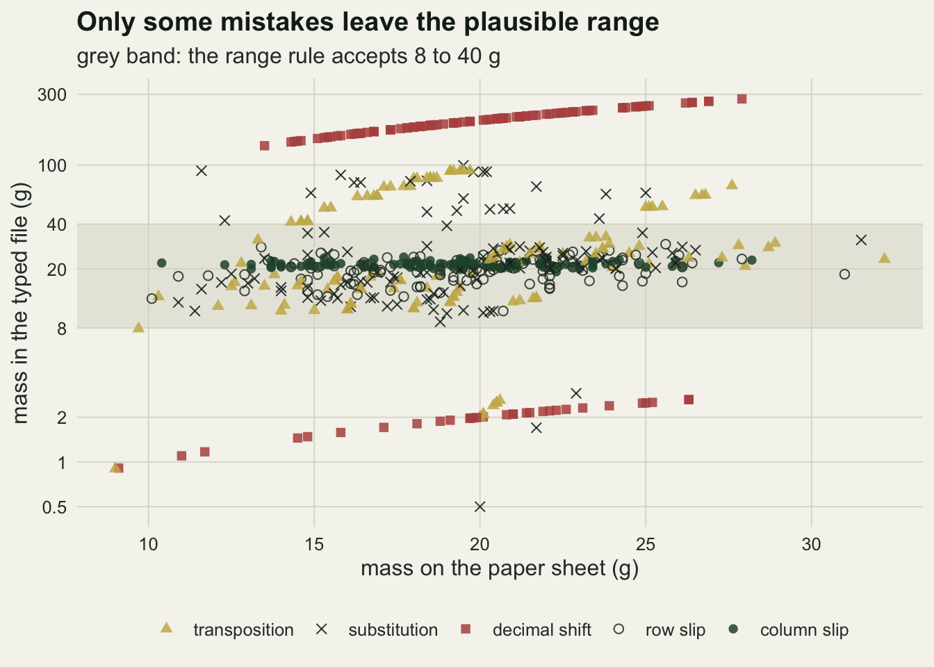
The figure pools 600 wrong fields. The decimal shifts sit far above and below the grey band, a factor of ten away from the true value. The column slips form a flat stripe at hind foot length, inside the band whatever the true mass was. The row slips scatter inside the band too, because a neighbour’s mass is a plausible mass. Transpositions split: a swap of the first two digits leaves the band when the new leading digit makes the mass 40 g or more or less than 8 g (18.4 to 81.4, 10.2 to 1.2, 9.5 to 5.9), and the rest stay in. Substitutions scatter in the same way but more widely: a changed leading digit can send the mass above the band or far below it, while a changed later digit keeps it close to the true value and inside.
What each check catches
run_checks <- function(p_err, q_share) {
  sheet <- make_sheet()
  k1 <- key_sheet(sheet, p_err)
  k2 <- key_sheet(sheet, p_err)
  wrong1 <- k1$typed != sheet$mass
  copied <- wrong1 & runif(n_row) < q_share
  typed2 <- k2$typed
  typed2[copied] <- k1$typed[copied]
  file_double <- ifelse(k1$typed == typed2, k1$typed, sheet$mass)
  flag_range  <- k1$typed < lo_mass | k1$typed > hi_mass
  file_range  <- ifelse(flag_range, sheet$mass, k1$typed)
  file_both   <- ifelse(file_double < lo_mass | file_double > hi_mass,
                        sheet$mass, file_double)
  ct <- true_contrast(sheet$mass, sheet$grazed)
  mech_f <- factor(k1$mech, levels = names(mech_share))
  per_mech <- function(keep) tabulate(mech_f[keep], nbins = length(mech_share))
  wt <- ifelse(sheet$grazed, -1, 1) / (n_row / 2) / ct
  left_range <- wrong1 & !flag_range
  c(wrong = per_mech(wrong1),
    range = per_mech(wrong1 & flag_range),
    double = per_mech(wrong1 & file_double == sheet$mass),
    shift_none   = true_contrast(k1$typed, sheet$grazed) / ct - 1,
    shift_range  = true_contrast(file_range, sheet$grazed) / ct - 1,
    shift_double = true_contrast(file_double, sheet$grazed) / ct - 1,
    shift_both   = true_contrast(file_both, sheet$grazed) / ct - 1,
    part = vapply(names(mech_share), function(m)
      sum(((k1$typed - sheet$mass) * wt)[left_range & k1$mech %in% m]), 0),
    contrast = ct)
}

n_rep <- 10000
set.seed(8192)
mc_out <- t(replicate(n_rep, run_checks(p_err_set, q_share_set)))

n_mech <- length(mech_share)
wrong_by  <- colSums(mc_out[, 1:n_mech])
range_by  <- colSums(mc_out[, n_mech + 1:n_mech])
double_by <- colSums(mc_out[, 2 * n_mech + 1:n_mech])
names(wrong_by) <- names(range_by) <- names(double_by) <- names(mech_share)
n_wrong_all  <- sum(wrong_by)
catch_range  <- sum(range_by) / n_wrong_all
catch_double <- sum(double_by) / n_wrong_all
se_catch_range  <- sqrt(catch_range * (1 - catch_range) / n_wrong_all)
se_catch_double <- sqrt(catch_double * (1 - catch_double) / n_wrong_all)
per_sheet_wrong <- n_wrong_all / n_rep
mech_share_seen <- wrong_by / n_wrong_all

catch_tab <- data.frame(
  mech  = rep(mech_label, 2),
  check = rep(c("range rule", "double entry"), each = n_mech),
  rate  = c(range_by / wrong_by, double_by / wrong_by))
catch_by_range  <- range_by / wrong_by
catch_by_double <- double_by / wrong_by
catch_tab$mech <- factor(catch_tab$mech,
  levels = rev(mech_label))
round(rbind(range = range_by / wrong_by, double = double_by / wrong_by), 3)
transposition substitution decimal row_slip column_slip
range 0.393 0.254 1.000 0.000 0.000
double 0.950 0.949 0.948 0.951 0.948Across 10000 keyed sheets the first keyer made 9.7 wrong masses per sheet on average, and 18.5 per cent of them were transpositions, a little under the design share of 20 because some swaps change nothing. The range rule caught 0.327 of all wrong fields and double entry caught 0.949 (Monte Carlo standard errors 0.0015 and 0.0007). On catch rate alone double entry wins by a wide margin, and a methods section that reports catch rates would say so.
ggplot(catch_tab, aes(rate, mech, colour = check, shape = check)) +
  geom_line(aes(group = mech), colour = te_line, linewidth = 1.2) +
  geom_point(size = 3.4) +
  scale_colour_manual(values = c("double entry" = te_forest, "range rule" = te_rust)) +
  scale_shape_manual(values = c("double entry" = 16, "range rule" = 17)) +
  scale_x_continuous(limits = c(0, 1), breaks = seq(0, 1, 0.2)) +
  labs(x = "share of wrong fields caught", y = NULL, colour = NULL, shape = NULL,
       title = "The range rule sees one kind of mistake",
       subtitle = "double entry sees nearly all of them, whatever the mechanism") +
  theme_datasheet() +
  theme(legend.position = "bottom")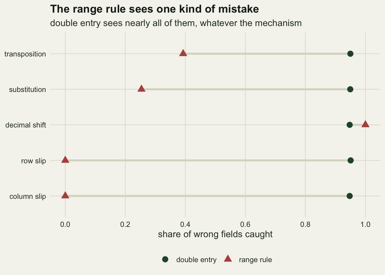
The mechanism view explains the totals. The range rule catches 1.000 of decimal shifts, 0.393 of transpositions, 0.254 of substitutions, 0.000 of row slips and 0.000 of column slips. Double entry catches between 0.948 and 0.951 of every mechanism, and what it misses is mostly the copied errors, at the set probability of 0.05. Its miss rate does not depend on what the error does to the number. The range rule’s miss rate depends on nothing else.
What the survivors do to the contrast
The quantity that matters for the survey is the ungrazed minus grazed difference in mean mass. For each sheet the shift is the contrast computed from the checked file divided by the contrast computed from the paper, minus one, so it is a relative error caused by typing alone and sampling variation does not enter it.
shift_cols <- c("shift_none", "shift_range", "shift_double", "shift_both")
shift_mean <- colMeans(mc_out[, shift_cols])
shift_mcse <- apply(mc_out[, shift_cols], 2, sd) / sqrt(n_rep)
shift_rms  <- sqrt(colMeans(mc_out[, shift_cols]^2))
shift_q99  <- apply(abs(mc_out[, shift_cols]), 2, quantile, probs = 0.99)
shift_neg  <- colMeans(mc_out[, shift_cols] < 0)
shift_zero <- colMeans(mc_out[, shift_cols] == 0)
part_mean  <- colMeans(mc_out[, paste0("part.", names(mech_share))])
names(part_mean) <- names(mech_share)
part_mcse  <- apply(mc_out[, paste0("part.", names(mech_share))], 2, sd) / sqrt(n_rep)
names(part_mcse) <- names(mech_share)
col_expect <- -100 * p_err_set * mech_share[["column_slip"]]
se_contrast <- sd(mc_out[, "contrast"])
se_contrast_rel <- se_contrast / (mu_ungrazed - mu_grazed)
n_big_double <- sum(abs(mc_out[, "shift_double"]) > 0.05)
n_big_range  <- sum(abs(mc_out[, "shift_range"]) > 0.05)
z_double   <- shift_mean[3] / shift_mcse[3]
n_over_se  <- sum(abs(mc_out[, "shift_double"]) > se_contrast_rel)
round(rbind(mean = shift_mean, mcse = shift_mcse, rms = shift_rms,
            q99 = shift_q99, negative = shift_neg, exact_zero = shift_zero), 5)
shift_none shift_range shift_double shift_both
mean 0.00784 -0.00249 0.00005 -0.00014
mcse 0.00148 0.00009 0.00033 0.00002
rms 0.14865 0.00903 0.03301 0.00201
q99 0.42766 0.02557 0.14509 0.00798
negative 0.49400 0.61040 0.21470 0.15830
exact_zero 0.00020 0.00320 0.60640 0.71910With no check at all, the typed contrast is off by 14.9 per cent in root mean square, almost entirely from the errors that leave the plausible range, decimal shifts above all: one dropped point adds nine times the true mass of that capture to its group total. The mean shift without a check is 0.78 per cent (Monte Carlo standard error 0.15); a dropped point in the heavier group adds more than one in the lighter group, but the mean is a poor summary of a spread this wide.
After the range rule the picture changes in kind. The mean shift is -0.249 per cent with a Monte Carlo standard error of 0.009, and the contrast is pulled towards zero in 61.0 per cent of sheets. The direction follows from what survives. A field the range rule accepts has been replaced by a value that is plausible but carries less information about treatment: the hind foot length carries none, a changed or swapped digit keeps part of it, and a neighbour’s mass keeps nearly all of it because the neighbour is almost always on the same plot. Replacing a value with something less tied to treatment pulls both group means towards a common value and shrinks the difference. Split by mechanism, column slips account for -0.199 percentage points of the mean shift, substitutions -0.009, transpositions -0.017 and row slips -0.024 (Monte Carlo standard errors up to 0.005); the three mechanisms that keep some link to treatment remove 0.050 points between them. Row slips show up at all only through the few that cross a plot boundary, where a mass from the other treatment is typed in. The column slips dominate because they are the only survivors with no link at all to treatment: each one replaces a mass by a value drawn from the same distribution in both groups, so in expectation it removes its own share of the contrast, 0.01 times 0.20, or 0.20 per cent, whatever the neighbouring column’s typical value. That value changes the spread of the shift, not its mean, and the expected size would be the same for any in range column that does not itself differ between treatments.
After double entry the mean shift is 0.005 per cent with a Monte Carlo standard error of 0.033, 0.2 standard errors from zero, and 60.6 per cent of sheets come out exactly right. So far that matches the case for double entry. The root mean square tells the other half: 3.30 per cent after double entry against 0.90 per cent after the range rule. The contrast is off by more than five per cent in 738 of the 10000 double entered sheets and in 0 of the range screened ones. Double entry misses few errors, but the ones it misses are a random draw from all mechanisms, and that includes the copied dropped decimal point, which is exactly the error the range rule never misses.
Running both checks, range rule on the double entered file, gives a root mean square shift of 0.20 per cent and a mean of -0.014 per cent. For scale, the sampling standard error of the contrast across these sheets is 0.221 g, or 7.4 per cent of the true difference of 3 g. At this error rate each of the three root mean square shifts is smaller than that sampling error; what the root mean square hides for double entry is that its value is an average over mostly exact sheets, some small shifts and 665 sheets in 10000 where the typing error alone is larger than the sampling error.
shift_long <- data.frame(
  check = factor(rep(c("range rule", "double entry", "both"), each = n_rep),
                 levels = c("range rule", "double entry", "both")),
  shift = 100 * c(mc_out[, "shift_range"], mc_out[, "shift_double"],
                  mc_out[, "shift_both"]))
shift_long$shown <- pmin(pmax(shift_long$shift, -8), 8)
ggplot(shift_long, aes(shown)) +
  geom_histogram(binwidth = 0.25, boundary = 0, fill = te_forest, colour = NA) +
  geom_vline(xintercept = 0, colour = te_rust, linewidth = 0.5) +
  facet_wrap(~ check, ncol = 1, scales = "free_y") +
  labs(x = "shift in the contrast (per cent of the true difference)",
       y = "sheets",
       title = "Small and left of zero, or mostly zero with a long tail",
       subtitle = "red line: no shift; outer bars collect every shift beyond eight per cent") +
  theme_datasheet()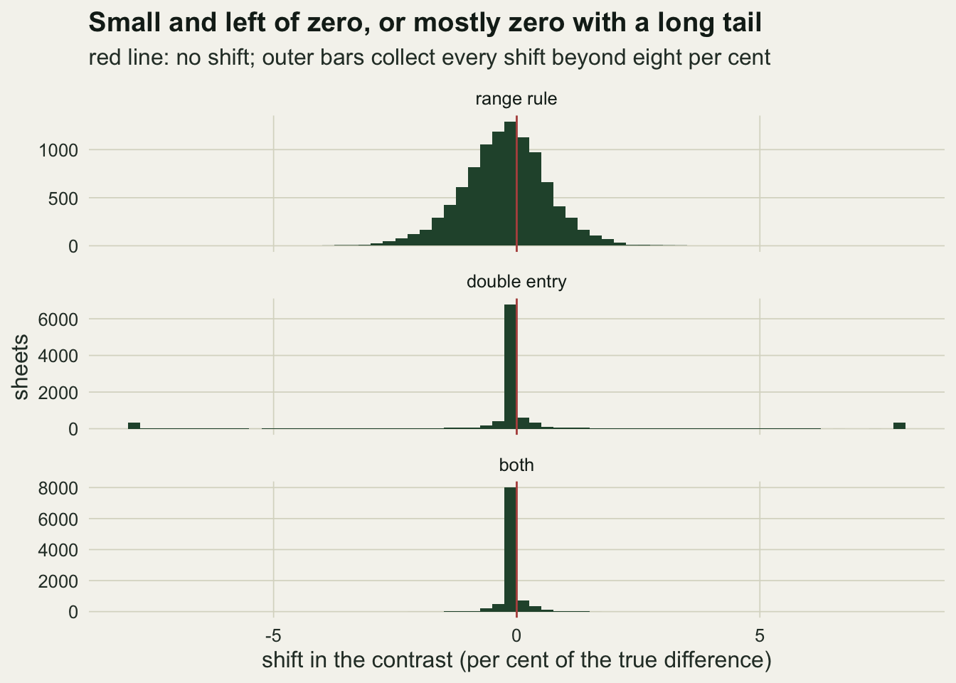
How much double entry depends on shared mistakes
The copying probability of 0.05 was a guess, and double entry’s residue is made of little else. The run below repeats the comparison for a range of copying probabilities, from zero (the keyers share nothing, and only chance coincidences survive) to one in five, and once more at a per field error rate five times lower, to see whether the ranking is a product of the chosen rate.
q_grid <- c(0, 0.01, 0.02, 0.05, 0.1, 0.2)
n_rep_grid <- 3000
rms_of <- function(x) sqrt(mean(x^2))
rms_se_of <- function(x) sd(x^2) / sqrt(length(x)) / (2 * sqrt(mean(x^2)))
set.seed(8193)
grid_out <- lapply(q_grid, function(q) t(replicate(n_rep_grid, run_checks(p_err_set, q))))
grid_rows <- lapply(seq_along(q_grid), function(g) {
  out <- grid_out[[g]]
  data.frame(q_share = q_grid[g],
             check = c("range rule", "double entry", "both"),
             rms = 100 * c(rms_of(out[, "shift_range"]),
                           rms_of(out[, "shift_double"]),
                           rms_of(out[, "shift_both"])),
             rms_se = 100 * c(rms_se_of(out[, "shift_range"]),
                              rms_se_of(out[, "shift_double"]),
                              rms_se_of(out[, "shift_both"])))
})
grid_tab <- do.call(rbind, grid_rows)
grid_tab$check <- factor(grid_tab$check, levels = c("range rule", "double entry", "both"))
rms_d_q0 <- grid_tab$rms[grid_tab$q_share == 0 & grid_tab$check == "double entry"]
rms_r_q0 <- grid_tab$rms[grid_tab$q_share == 0 & grid_tab$check == "range rule"]
se_d_q0 <- grid_tab$rms_se[grid_tab$q_share == 0 & grid_tab$check == "double entry"]
se_r_q0 <- grid_tab$rms_se[grid_tab$q_share == 0 & grid_tab$check == "range rule"]
z_q0 <- (rms_r_q0 - rms_d_q0) / sqrt(se_d_q0^2 + se_r_q0^2)
rms_d_q01 <- grid_tab$rms[grid_tab$q_share == 0.01 & grid_tab$check == "double entry"]
rms_r_q01 <- grid_tab$rms[grid_tab$q_share == 0.01 & grid_tab$check == "range rule"]
rms_d_q20 <- grid_tab$rms[grid_tab$q_share == 0.2 & grid_tab$check == "double entry"]
out_q0 <- grid_out[[which(q_grid == 0)]]
miss_q0_by <- colSums(out_q0[, 1:n_mech]) - colSums(out_q0[, 2 * n_mech + 1:n_mech])
names(miss_q0_by) <- names(mech_share)
miss_q0 <- sum(miss_q0_by) / sum(out_q0[, 1:n_mech])

p_err_low <- 0.002
set.seed(8194)
low_out <- t(replicate(n_rep_grid, run_checks(p_err_low, q_share_set)))
rms_low_range  <- 100 * rms_of(low_out[, "shift_range"])
rms_low_double <- 100 * rms_of(low_out[, "shift_double"])
ratio_set <- shift_rms[3] / shift_rms[2]
ratio_low <- rms_low_double / rms_low_range
se_low_range  <- 100 * rms_se_of(low_out[, "shift_range"])
se_low_double <- 100 * rms_se_of(low_out[, "shift_double"])
se_ratio_low <- ratio_low * sqrt((se_low_double / rms_low_double)^2 +
                                 (se_low_range / rms_low_range)^2)
miss_q0_by
transposition substitution decimal row_slip column_slip
2 1 8 6 11 grid_tab q_share check rms rms_se
1 0.00 range rule 0.90442950 0.014060720
2 0.00 double entry 0.45707378 0.103878114
3 0.00 both 0.02429923 0.008936037
4 0.01 range rule 0.90450952 0.013799983
5 0.01 double entry 1.66726063 0.114480512
6 0.01 both 0.08596137 0.007269727
7 0.02 range rule 0.89957206 0.013391788
8 0.02 double entry 2.07259729 0.131436453
9 0.02 both 0.12571514 0.006319160
10 0.05 range rule 0.88802857 0.012978136
11 0.05 double entry 3.31617653 0.128091703
12 0.05 both 0.19866709 0.007706181
13 0.10 range rule 0.90792513 0.014060050
14 0.10 double entry 4.65366645 0.120024003
15 0.10 both 0.28705101 0.007480114
16 0.20 range rule 0.92380221 0.013948004
17 0.20 double entry 6.86662430 0.161885670
18 0.20 both 0.39215139 0.008222309ggplot(grid_tab, aes(q_share, rms, colour = check, shape = check)) +
geom_line(linewidth = 0.9) +
geom_errorbar(aes(ymin = rms - 2 * rms_se, ymax = rms + 2 * rms_se),
width = 0.004, linewidth = 0.5) +
geom_point(size = 2.8) +
scale_colour_manual(values = c("range rule" = te_rust, "double entry" = te_forest,
"both" = te_gold)) +
scale_shape_manual(values = c("range rule" = 17, "double entry" = 16, "both" = 15)) +
labs(x = "probability the second keyer copies a mistake",
y = "root mean square shift (per cent)", colour = NULL, shape = NULL,
title = "Double entry is only as good as its keyers are independent",
subtitle = "per field error rate 0.01; the range rule does not depend on the second keyer") +
theme_datasheet() +
theme(legend.position = "bottom")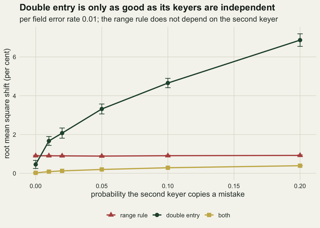
With fully independent keyers double entry leaves a root mean square shift of 0.46 per cent (Monte Carlo standard error 0.10) against 0.90 per cent (0.01) for the range rule, 4.3 standard errors apart. That standard error is a rough guide only, because what double entry leaves with independent keyers is chance coincidence, and in these 3000 sheets it came to 28 fields: most often both keyers typing the neighbouring column (11), which is harmless in size, and 8 coincident decimal shifts, which are not, so a handful of sheets sets the whole root mean square. Because a coincident decimal shift needs both keyers to pick that mechanism, their number goes with the square of the decimal share, and this one comparison depends strongly on the assumed mechanism mix. A little sharing reverses the order. At a copying probability of 0.01 the two stand at 1.67 and 0.90 per cent, and at 0.2 double entry reaches 6.87 per cent. The combined check stays lowest across the whole range, since the range rule removes precisely the shared errors that do the damage.
Lowering the per field error rate to 0.002 shrinks everything, to 0.38 per cent after the range rule and 1.37 per cent after double entry, but the ratio of the two root mean square shifts moves only from 3.65 to 3.62 (Monte Carlo standard error of the second 0.31). Both residues come from a count of surviving errors that scales with the rate as long as copied mistakes outnumber chance coincidences. With independent keyers at the set rate, 0.0010 of wrong fields survived double entry by coincidence, while copied mistakes survive in a share equal to the copying probability, so above a copying probability of about that size the rate sets the size of the problem and the copying probability and the mechanism mix set the ranking. With fully independent keyers the number of coincidences falls with the square of the rate while the number of range rule survivors falls in proportion to it, so double entry’s lead at a copying probability of zero, seen in the last figure, would widen in relative terms at lower rates.
What to report
Report which checks were run, in the order they were run, and do not report a catch rate as if it described the quality of the data. A catch rate is measured against the errors a check can see; the range rule in this simulation catches 0.327 of wrong fields and leaves a file whose contrast is shifted towards zero on average, and double entry catches 0.949 and leaves a file that is more often than not exact and occasionally badly wrong.
If double entry is used, report the disagreement rate between keyers. Half of it is the most direct estimate of the per field error rate of one keyer, and the rate can be turned into an expected number of undetected errors once a copying probability is assumed. If the second keyer worked from the first keyer’s file rather than from the paper, the two are not independent and the procedure is visual checking with extra steps.
Run a range rule on every double entered file. It costs nothing, it catches the out of range errors that double entry lets through when both keyers fail on the same field, and in this simulation it cut the root mean square shift from 3.30 to 0.20 per cent.
When only a range rule was possible, say so next to the effect estimate, and name the columns adjacent to the response on the entry form. A column slip from a neighbouring variable is invisible to a range rule when that variable’s values lie inside the limits, and it did most of the damage among the survivors here; it removes its own share of the contrast wherever the neighbour’s values sit, and more or less than that if the neighbouring variable itself differs between treatments.
Honest limits
The error model is invented. The five mechanisms are common in spreadsheets typed from paper, but the set is not complete and no source cited here lists it: unit errors are folded into decimal shifts, substitutions are drawn uniformly rather than between look-alike digits, and whole skipped or duplicated rows are absent. Their shares, the per field rate and the copying probability were chosen, not estimated. The findings that do not depend on those choices are structural: a range rule’s survivors are the in range errors, and to the extent they lose their link to treatment they attenuate a contrast; double entry’s survivors are a sample of all mechanisms whose size is set by how often keyers share a mistake.
The copying probability applies equally to every mechanism. In reality shared errors are more likely from an unclear handwritten digit than from a dropped decimal point, which is a keying slip one person makes and another usually does not. If copied errors are mostly small misreadings, double entry’s long tail shrinks and its advantage returns sooner than the last figure suggests.
Only one column is keyed with error and only one analysis is examined. Errors in the treatment or plot column would misassign whole captures, which a range rule cannot see at all, and a regression on body mass with hind foot as a covariate would be affected by errors in both columns at once. Contrast attenuation is the answer for a difference in means; a variance, a maximum or a correlation responds to the same survivors differently.
The checks here are perfect when they fire: every flagged or disagreeing value is corrected to the truth. Looking up a value on a sheet that is itself hard to read can fail, and that failure would hit both checks.
References
Barchard KA, Pace LA 2011 Computers in Human Behavior 27(5):1834-1839 (10.1016/j.chb.2011.04.004)
Day S, Fayers P, Harvey D 1998 Controlled Clinical Trials 19(1):15-24 (10.1016/S0197-2456(97)00096-2)
Paulsen A, Overgaard S, Lauritsen JM 2012 PLoS ONE 7(4):e35087 (10.1371/journal.pone.0035087)