library(ggplot2)

te_pal <- list(forest = "#275139", green = "#2f8f63", sage = "#93a87f",
               clay = "#b5534e", gold = "#cda23f", line = "#dad9ca",
               ink = "#16241d", paper = "#f5f4ee")

theme_te <- function() {
  theme_minimal(base_size = 12) +
    theme(panel.grid.minor = element_blank(),
          panel.grid.major = element_line(colour = "#e7e6dc"),
          plot.background = element_rect(fill = "#f5f4ee", colour = NA),
          panel.background = element_rect(fill = "#f5f4ee", colour = NA),
          plot.title = element_text(face = "bold", colour = te_pal$ink),
          axis.title = element_text(colour = "#2c3a31"),
          axis.text = element_text(colour = "#2c3a31"))
}Robust regression for ecological outliers
R
regression
MASS
ecology tutorial
An outlier is a claim about the model, not about the point. Measuring leverage, breakdown points and the real price of robust regression on grassland data.
A chalk grassland survey: one hundred and twenty permanent plots, a soil core from each sent away for available nitrogen, and a peak-season harvest clipped, dried and weighed. Biomass rises with nitrogen, a straight line through the scatter is the whole analysis, and the slope goes in the paper. Then the field notebook turns up two plots with a question mark against them. One plot sits on an old sheep fold where the soil nitrogen is three times anything else in the survey. One plot was clipped with the small quadrat frame and nobody wrote that down, so its recorded harvest is too low.
The reflex is to plot the data, find the points that sit far from the fitted line, and drop them. That procedure is circular, and the circularity is the whole problem: the line was fitted with those points in it, so the residuals it hands back are already a compromise between the bulk of the data and whatever is wrong with the suspects. A point that pulled the line onto itself has a small residual, and a point that could not move the line at all has a large one. Neither residual is telling you what you want to know.
The question worth asking is not which points are outliers. An outlier is a claim about the model, not about the point: it says that this observation and the rest of the data cannot both have come from the same process. The useful version of that claim is quantitative, and it has two halves. How much of my slope rests on this point, and is there a way to fit the line that does not let a handful of observations decide the answer.
This post measures four things. What the standard influence diagnostics say about three different ways of being unusual, and where they mislead. How much contamination each estimator survives before its answer is worthless, measured rather than quoted. What the insurance premium is on clean data, in standard errors. And the three situations in which robust regression returns a confident wrong answer, one of which cannot be detected from the data at all.
Two neighbouring posts ask nearby questions and are not this one. Quantile regression fits the conditional median, which does resist contamination in the response, but it is aimed at a different target: a conditional quantile is a statement about where a fraction of the distribution sits, whereas everything below is trying to recover a conditional mean without letting a few observations own it. Measurement error and regression dilution deals with error in the predictor, which is a separate problem with a separate fix; nothing here helps with it. And GLM residual diagnostics builds residual checks for models where the residual itself is hard to read. The material below is plain Gaussian regression, where the residual is easy to read and still misleading.
Three ways a plot can be unusual
The survey is synthetic, so the truth is known and every error below is a distance from a number that was set rather than an argument about what should have happened. Biomass is generated as a straight line in soil nitrogen with Gaussian noise, and then three separate copies of the dataset are made, each carrying exactly one contaminated plot.
library(MASS)

n_plot <- 120
b0 <- 120
b1 <- 4.5
sig_e <- 18

set.seed(20260801)
nit <- rnorm(n_plot, 40, 7)
bio <- b0 + b1 * nit + rnorm(n_plot, 0, sig_e)
clean <- data.frame(nitrogen = nit, biomass = bio)
fit_clean <- lm(biomass ~ nitrogen, data = clean)

slip <- -250
x_far <- 120
i_v <- which.min(abs(nit - mean(nit)))
i_x <- 2

make_case <- function(kind) {
  d <- clean
  if (kind == "vertical") {
    d$biomass[i_v] <- d$biomass[i_v] + slip
  } else {
    d$nitrogen[i_x] <- x_far
    d$biomass[i_x] <- b0 + b1 * x_far + 6 + (kind == "bad") * slip
  }
  d
}

print(round(c(plots = n_plot, true_intercept = b0, true_slope = b1,
              residual_sd = sig_e, recording_slip = slip,
              sheepfold_nitrogen = x_far,
              fitted_slope = unname(coef(fit_clean)[2]),
              fitted_se = summary(fit_clean)$coefficients[2, 2],
              fitted_sigma = summary(fit_clean)$sigma), 4))
plots true_intercept true_slope residual_sd
120.0000 120.0000 4.5000 18.0000
recording_slip sheepfold_nitrogen fitted_slope fitted_se
-250.0000 120.0000 4.5269 0.2254
fitted_sigma
17.8963 The clean survey returns a slope of 4.5269 grams of biomass per square metre per milligram of nitrogen per kilogram of soil, against a true value of 4.5, with a standard error of 0.2254. That is the answer the three contaminated copies have to be judged against.
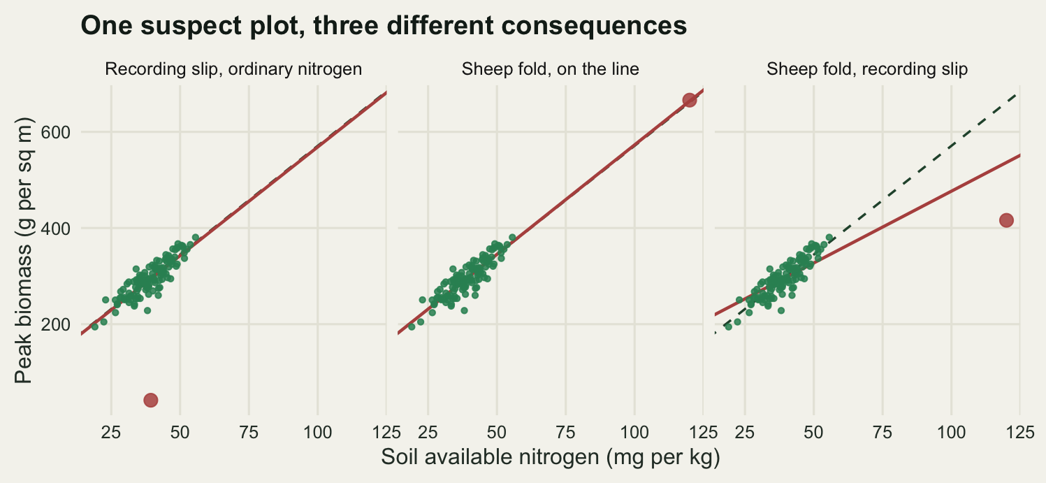
The recording slip is the same in two of the three: 250 grams of biomass per square metre subtracted from one plot. In the first copy the affected plot has an ordinary soil nitrogen value, close to the survey mean. In the third copy it is the sheep fold plot, at 120 milligrams per kilogram against a survey mean of 39.25. The second copy is the control: the sheep fold plot is there, its nitrogen is just as extreme, and its biomass follows the same line as everything else.
Three quantities describe what any single observation does to a straight-line fit. The first is leverage, the capacity of a plot to pull the line towards itself, which comes entirely from where it sits along the predictor and not at all from its response. Its measure is the hat value \(h_i\), the \(i\)th diagonal element of \(H = X(X^\top X)^{-1}X^\top\), scaled so that the whole set adds up to the number of coefficients. The standardised residual divides the raw residual by its own standard deviation, \(\hat\sigma\sqrt{1 - h_i}\). Cook’s distance combines the two and reports how far all the fitted values move when the observation is dropped. Leverage is not influence: a high-leverage point can leave the fit exactly where it was, and the three copies below are built to separate them.
Xm <- model.matrix(fit_clean)
Hm <- Xm %*% solve(crossprod(Xm)) %*% t(Xm)
hat_hand <- diag(Hm)
e_cl <- residuals(fit_clean)
s_cl <- sqrt(sum(e_cl^2) / (n_plot - 2))
rstd_hand <- e_cl / (s_cl * sqrt(1 - hat_hand))
cook_hand <- rstd_hand^2 / 2 * hat_hand / (1 - hat_hand)

print(round(c(hat_gap = max(abs(hat_hand - hatvalues(fit_clean))),
              rstd_gap = max(abs(rstd_hand - rstandard(fit_clean))),
              cook_gap = max(abs(cook_hand - cooks.distance(fit_clean)))), 12))
hat_gap rstd_gap cook_gap
0 0 0 case_row <- function(kind) {
i <- if (kind == "vertical") i_v else i_x
d <- make_case(kind)
f <- lm(biomass ~ nitrogen, data = d)
f_drop <- lm(biomass ~ nitrogen, data = d[-i, ])
c(hat = unname(hatvalues(f)[i]),
residual = unname(residuals(f)[i]),
deleted_residual = unname(d$biomass[i] - predict(f_drop, d[i, ])),
std_residual = unname(rstandard(f)[i]),
cooks_d = unname(cooks.distance(f)[i]),
slope = unname(coef(f)[2]),
slope_dropped = unname(coef(f_drop)[2]),
slope_se = summary(f)$coefficients[2, 2],
sigma = summary(f)$sigma)
}
cases <- rbind(vertical = case_row("vertical"),
good = case_row("good"),
bad = case_row("bad"))
print(round(cases, 4)) hat residual deleted_residual std_residual cooks_d slope
vertical 0.0083 -252.7203 -254.8447 -8.6244 0.3126 4.5219
good 0.5106 1.8694 3.8201 0.1512 0.0119 4.5553
bad 0.5106 -120.4710 -246.1799 -7.2550 27.4617 2.9873
slope_dropped slope_se sigma
vertical 4.5270 0.3707 29.4259
good 4.5313 0.1564 17.6687
bad 4.5313 0.2101 23.7373print(round(c(average_hat = 2 / n_plot,
largest_clean_hat = max(hatvalues(fit_clean)),
deflation_bad = 1 / (1 - cases["bad", "hat"]),
deflation_vertical = 1 / (1 - cases["vertical", "hat"])), 4)) average_hat largest_clean_hat deflation_bad deflation_vertical
0.0167 0.0730 2.0435 1.0084 The hand-built hat matrix, standardised residual and Cook’s distance agree with the built-in functions to the last digit R prints, which is worth checking once because the formulae are the argument of this section rather than a black box.
Read the table by columns. The plot with the recording slip at ordinary nitrogen is a low-leverage point, hat value 0.0083 against an average of 0.0167, and it has a standardised residual of -8.624, which is the largest in the dataset by a wide margin. It is the most conspicuous point in any residual plot you could draw. It is also almost harmless to the slope: the fit gives 4.5219 with the plot in and 4.527 with it out, a change of -0.0051. What it does damage is precision. The residual standard deviation goes from 17.896 to 29.426, and the standard error on the slope from 0.2254 to 0.3707, a rise of 64.4 per cent.
The sheep fold plot in the second copy has a hat value of 0.5106, 31 times the average and 7 times the largest hat value anywhere in the clean survey. The usual rule of thumb for flagging high-leverage points is twice the average hat value, a cut-off that goes back to Hoaglin and Welsch (1978), and this plot is caught by it immediately. Nothing is wrong with it. Its standardised residual is 0.1512, its Cook’s distance is 0.0119, the slope moves from 4.5313 to 4.5553 when it is added, and the standard error falls from 0.2254 to 0.1564. The literature calls this a good leverage point: extreme in the predictor and obedient to the same relationship, which makes it the most informative observation in the survey, worth 30.6 per cent off the standard error on its own. A rule that deletes high-leverage points on sight throws away the best plot in the dataset.
The third copy is the one that matters, and it is the bad leverage point: the same sheep fold plot at the same hat value of 0.5106, now carrying the same recording slip of 250 grams as the first copy. The slope collapses from 4.5313 to 2.9873, an attenuation of 34.1 per cent, and Cook’s distance is 27.46, against 0.313 for the conspicuous plot in the first copy.
Now the part that makes residual-hunting circular. The recording error is identical in the two copies, and yet the residual it produces is not. In the first copy the residual is -252.7 grams, essentially the whole error. In the third copy it is -120.5 grams, only 48.2 per cent of it. Measured against the line fitted from the other 119 plots, the same error shows up as -246.2 grams. The ratio of the two is \(1/(1 - h_i) =\) 2.043: the plot dragged the line 2.04 times closer to itself than an ordinary plot at the same distance from it could have, and hid half its own error while doing it.
One weighted least squares loop
The alternative to deciding what to delete is to fit the line in a way that gives every observation a weight, and to let the weight depend on how badly the observation disagrees with the fit. That is circular too, so it is done by iteration: fit, compute residuals, set weights, refit, until the coefficients stop moving.
Huber’s proposal is to weight an observation by one if its scaled residual is small and by \(k/|u_i|\) if it is large, with \(u_i = r_i/\hat s\) and \(\hat s\) a scale estimate that is itself resistant, here the median absolute residual divided by 0.6745. The effect is that a point five scale units away contributes as much to the normal equations as a point \(k\) units away, and no more. The loop is short enough to write out, and writing it out is the point: rlm is not doing anything a reader cannot check.
irls_huber <- function(X, y, k = 1.345, maxit = 60, tol = 1e-10) {
  bhat <- qr.solve(X, y)
  for (it in seq_len(maxit)) {
    r <- as.vector(y - X %*% bhat)
    s_rob <- median(abs(r)) / 0.6745
    w <- pmin(1, k * s_rob / abs(r))
    bnew <- solve(crossprod(X * w, X), crossprod(X * w, y))
    if (max(abs(bnew - bhat)) < tol) {
      bhat <- bnew
      break
    }
    bhat <- bnew
  }
  list(coef = as.vector(bhat), weights = w, iterations = it, scale = s_rob)
}

d_bad <- make_case("bad")
X_bad <- cbind(1, d_bad$nitrogen)
hand <- irls_huber(X_bad, d_bad$biomass)
mass_hub <- rlm(biomass ~ nitrogen, data = d_bad)

print(round(c(hand_intercept = hand$coef[1], hand_slope = hand$coef[2],
              rlm_intercept = unname(coef(mass_hub)[1]),
              rlm_slope = unname(coef(mass_hub)[2]),
              iterations = hand$iterations,
              hand_scale = hand$scale, rlm_scale = mass_hub$s,
              coef_gap = max(abs(hand$coef - coef(mass_hub))),
              weight_gap = max(abs(hand$weights - mass_hub$w))), 6))
hand_intercept hand_slope rlm_intercept rlm_slope iterations
131.644755 4.207215 131.646418 4.207167 23.000000
hand_scale rlm_scale coef_gap weight_gap
19.644429 19.646030 0.001662 0.000111 The hand-written loop converges in 23 iterations to a slope of 4.2072 and rlm returns 4.2072; the largest disagreement across both coefficients is 0.00166 and across all 120 weights it is 0.000111, the residue of rlm stopping on a relative tolerance rather than running the loop to numerical convergence.
Two more estimators join the comparison. rlm with method = "MM" starts from a high-breakdown initial fit and then applies a redescending bisquare weight, which sends a badly disagreeing observation to exactly zero weight rather than merely reducing it; Yohai (1987) introduced that two-stage construction, and proved that it keeps the breakdown point of the starting fit while recovering most of the efficiency of least squares. lqs with method = "lts" fits least trimmed squares: it searches for the subset containing half the observations whose least squares fit has the smallest residual sum of squares, and ignores the rest entirely, which is one of the two estimators Rousseeuw (1984) put forward when he set out to reach a breakdown point of a half. Both involve a search over subsets, so both need a seed; nsamp = "exact" makes the least trimmed squares search deterministic at this sample size. Both functions come from MASS, and Venables and Ripley (2002) is the volume that documents what each of their arguments does.
four_fits <- function(d) {
  c(OLS = unname(coef(lm(biomass ~ nitrogen, data = d))[2]),
    Huber = unname(coef(rlm(biomass ~ nitrogen, data = d, maxit = 200))[2]),
    MM = unname(coef(rlm(biomass ~ nitrogen, data = d,
                         method = "MM", maxit = 200))[2]),
    LTS = unname(coef(lqs(biomass ~ nitrogen, data = d,
                          method = "lts", nsamp = "exact"))[2]))
}
set.seed(3030)
compare <- rbind(uncontaminated = four_fits(clean),
                 vertical = four_fits(make_case("vertical")),
                 good = four_fits(make_case("good")),
                 bad = four_fits(make_case("bad")))
print(round(compare, 4))
OLS Huber MM LTS
uncontaminated 4.5269 4.5704 4.5802 5.0971
vertical 4.5219 4.5663 4.5783 5.0933
good 4.5553 4.5700 4.5752 5.0971
bad 2.9873 4.2072 4.5839 5.0971print(round(compare - b1, 4)) OLS Huber MM LTS
uncontaminated 0.0269 0.0704 0.0802 0.5971
vertical 0.0219 0.0663 0.0783 0.5933
good 0.0553 0.0700 0.0752 0.5971
bad -1.5127 -0.2928 0.0839 0.5971On the copy that broke least squares, the Huber fit recovers 4.2072 and the MM fit 4.5839 against a truth of 4.5, where least squares returned 2.9873. Least trimmed squares gives 5.0971, and the interesting thing about that number is that it is 5.0971 on the uncontaminated survey as well. It is not reacting to the contamination; it is 0.57 away from the least squares answer on clean data, which is a preview of the third section.
The breakdown point, measured
The breakdown point of an estimator is the smallest fraction of the sample that has to be replaced by arbitrary values to send the estimate anywhere the contaminator likes. For least squares it is zero, asymptotically, and one observation in finite samples: take any single plot and move its recorded biomass, and the slope traces a straight line with no bound at either end.
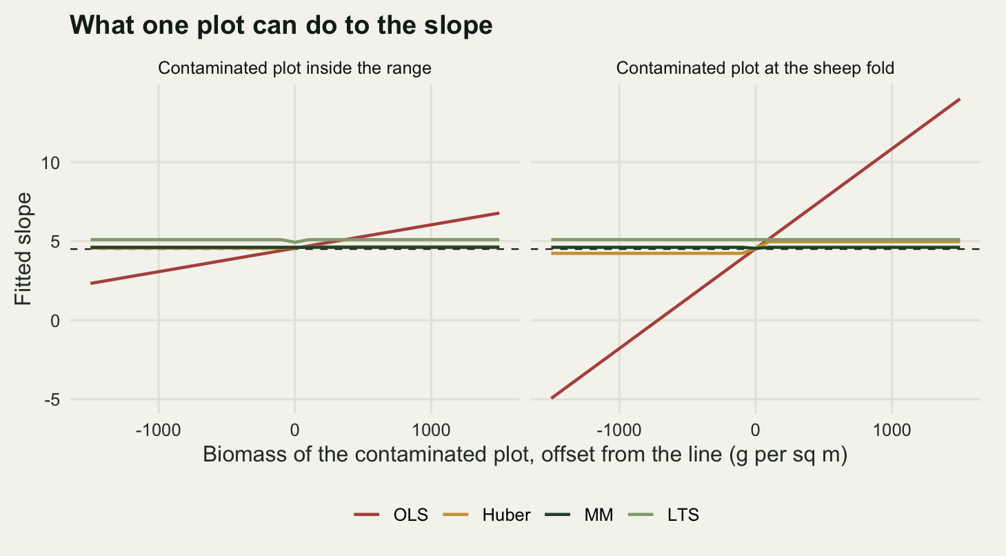
The first experiment does exactly that. One plot’s biomass is swept across a wide grid, twice over: once with the plot left at its own nitrogen value, inside the range of the survey, and once with it relocated to the sheep fold value outside the range.
i_s <- which.min(abs(nit - quantile(nit, 0.9)))
shift_grid <- seq(-1500, 1500, by = 100)

sweep_one <- function(x_pos) {
  out <- matrix(NA_real_, length(shift_grid), 4)
  for (j in seq_along(shift_grid)) {
    d <- clean
    d$nitrogen[i_s] <- x_pos
    d$biomass[i_s] <- b0 + b1 * x_pos + shift_grid[j]
    out[j, ] <- four_fits(d)
  }
  colnames(out) <- c("OLS", "Huber", "MM", "LTS")
  as.data.frame(out)
}
set.seed(5150)
sweep_in <- sweep_one(nit[i_s])
sweep_out <- sweep_one(x_far)

span <- function(z) diff(range(z))
print(round(c(swept_nitrogen = nit[i_s], shift_from = min(shift_grid),
              shift_to = max(shift_grid)), 3))
swept_nitrogen shift_from shift_to
48.592 -1500.000 1500.000 print(round(rbind(inside = sapply(sweep_in, span),
outside = sapply(sweep_out, span)), 4)) OLS Huber MM LTS
inside 4.4491 0.0799 0.0004 0.1693
outside 18.9446 0.7362 0.0652 0.0000print(round(c(ols_lowest = min(sweep_out$OLS), ols_highest = max(sweep_out$OLS),
huber_bound_ratio = span(sweep_out$Huber) / span(sweep_in$Huber)), 4)) ols_lowest ols_highest huber_bound_ratio
-4.9430 14.0016 9.2182 With the moved plot inside the range of the survey, at a nitrogen value of 48.59, the least squares slope travels 4.449 units across the grid while the Huber fit moves 0.0799, the MM fit 0.00043 and the least trimmed squares fit 0.1693. Moving the same plot out to the sheep fold nitrogen value changes the picture. Least squares now travels 18.945 units, from -4.943 to 14.002: one plot in 120 is enough to reverse the sign of the relationship between soil nitrogen and biomass. The Huber fit is still bounded, but its bound has widened by a factor of 9.22. That is the exact sense in which a monotone M-estimator has bounded influence in the response and none in the predictor: the weight caps what the residual can contribute, and then the leverage of the plot multiplies it back up.
One point is the easy case. The second experiment raises the number of contaminated plots from none to 54, close to half the survey, under two contamination geometries. In the first, the contaminated plots keep their soil nitrogen and have their biomass replaced by a value far above anything the relationship could produce, which is what a stuck balance or a misplaced decimal point looks like. In the second, they are moved out to high nitrogen as well, which is what a systematically mishandled group of plots looks like: the sheep fold transect sampled with the wrong frame, a batch of soil cores analysed at a different lab.
k_grid <- 0:54

contaminate <- function(k, mode) {
  d <- clean
  if (k == 0) return(d)
  set.seed(90900 + 100 * (mode == "highx") + k)
  ii <- seq_len(k)
  if (mode == "highx") {
    d$nitrogen[ii] <- rnorm(k, 110, 6)
    d$biomass[ii] <- rnorm(k, 250, 18)
  } else {
    d$biomass[ii] <- rnorm(k, 950, 20)
  }
  d
}

run_fraction <- function(mode) {
  out <- matrix(NA_real_, length(k_grid), 4)
  for (j in seq_along(k_grid)) {
    d <- contaminate(k_grid[j], mode)
    set.seed(600 + k_grid[j])
    out[j, ] <- four_fits(d)
  }
  colnames(out) <- c("OLS", "Huber", "MM", "LTS")
  as.data.frame(out)
}
frac_vert <- run_fraction("vert")
frac_high <- run_fraction("highx")

break_at <- function(m) apply(m, 2, function(z) {
  bad <- which(abs(z - b1) > b1 / 2)
  if (!length(bad)) NA_real_ else 100 * k_grid[min(bad)] / n_plot
})
brk <- rbind(vertical = break_at(frac_vert), high_nitrogen = break_at(frac_high))
print(round(brk, 3))
OLS Huber MM LTS
vertical 4.167 32.500 NA NA
high_nitrogen 1.667 4.167 33.333 33.333print(round(cbind(percent = 100 * k_grid / n_plot, frac_high)[1:8, ], 3)) percent OLS Huber MM LTS
1 0.000 4.527 4.570 4.580 5.097
2 0.833 2.617 4.285 4.597 5.166
3 1.667 1.210 3.877 4.600 5.166
4 2.500 1.027 3.639 4.595 5.149
5 3.333 0.637 2.948 4.631 5.149
6 4.167 0.356 1.354 4.591 4.887
7 5.000 0.197 0.583 4.597 5.099
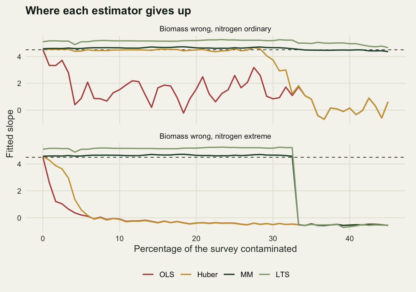
8 5.833 0.108 0.169 4.637 5.099Breakdown here is defined as the first contamination fraction at which the fitted slope misses the truth by more than half the truth, which for these data means leaving the band between 2.25 and 6.75. Against the pure response contamination, least squares breaks at 4.17 per cent of the survey, the Huber fit breaks at 32.5 per cent, and the MM and least trimmed squares fits never break within the range tested, still returning 4.363 and 4.658 with 45 per cent of the survey replaced.
Moving the same contamination out in the predictor cuts every one of those numbers. Least squares breaks at 1.67 per cent, which is 2 plots out of 120. The Huber fit breaks at 4.17 per cent, 7.8 times sooner than it did against response contamination, which is the practical meaning of a breakdown point of zero under contamination in the predictor. The MM and least trimmed squares fits fail together at the same step, at 33.33 per cent.
That shared failure point is below the fifty per cent both estimators are advertised as reaching, and the reason is worth measuring rather than asserting. An S-estimator, which is what the MM fit starts from, chooses the line that minimises a resistant measure of scale built from the residuals: the solution of \(\frac{1}{n}\sum \rho(r_i/s) = \tfrac12\) for the bisquare \(\rho\). Fifty per cent is a guarantee against the worst an adversary can do with that many points, not a promise about any particular pattern, and here the contaminated plots are a compact cloud rather than scattered noise. Compute that scale at the true line and at the line the estimator picked, one step before the failure and at it.
m_scale <- function(r, k0 = 1.548, b_cons = 0.5) {
  rho <- function(u) {
    z <- pmin(abs(u) / k0, 1)
    3 * z^2 - 3 * z^4 + z^6
  }
  uniroot(function(s) mean(rho(r / s)) - b_cons,
          c(1e-6, 10 * max(abs(r)) + 1))$root
}
k_break <- round(brk["high_nitrogen", "MM"] * n_plot / 100)

scale_pair <- function(k) {
  d <- contaminate(k, "highx")
  set.seed(600 + k)
  f <- rlm(biomass ~ nitrogen, data = d, method = "MM", maxit = 200)
  r_true <- d$biomass - (b0 + b1 * d$nitrogen)
  c(plots = k, percent = 100 * k / n_plot, slope = unname(coef(f)[2]),
    scale_true_line = m_scale(r_true), scale_fitted = m_scale(residuals(f)),
    ratio = m_scale(residuals(f)) / m_scale(r_true))
}
tie <- rbind(scale_pair(k_break - 1), scale_pair(k_break))
print(round(tie, 4))
plots percent slope scale_true_line scale_fitted ratio
[1,] 39 32.5000 4.5806 30.0529 30.1118 1.0020
[2,] 40 33.3333 -0.5309 30.7401 27.9284 0.9085One step before the failure, at 39 contaminated plots, the MM fit still returns 4.581 and the line it chose has a resistant scale of 30.112 against 30.053 at the true line, a gap of 0.2 per cent. One plot later the fit returns -0.531, and the line through both clouds now has a scale of 27.928 against 30.74.
The price of the insurance
Nothing above is free. On data that really are Gaussian, least squares is the efficient estimator and anything that down-weights an observation is throwing away information. The question is how much, and the answer is measurable: fit the same simulated survey many times over with each estimator and compare the spread of the estimates.
The design is a smaller survey, 60 plots with the predictor held fixed across replicates so that only the errors are redrawn. Three error regimes: clean Gaussian, and then 5 and 10 per cent of plots given a biomass error of six to ten residual standard deviations in a random direction, which is a recording slip rather than a heavy tail.
n_eff <- 60
set.seed(4411)
x_eff <- rnorm(n_eff, 40, 7)

one_replicate <- function(c_frac) {
  y <- b0 + b1 * x_eff + rnorm(n_eff, 0, sig_e)
  k <- round(c_frac * n_eff)
  if (k > 0) {
    ii <- sample.int(n_eff, k)
    y[ii] <- y[ii] + sample(c(-1, 1), k, TRUE) * runif(k, 6, 10) * sig_e
  }
  d <- data.frame(nitrogen = x_eff, biomass = y)
  f_ols <- lm(biomass ~ nitrogen, data = d)
  f_hub <- rlm(biomass ~ nitrogen, data = d, maxit = 200)
  f_mm <- rlm(biomass ~ nitrogen, data = d, method = "MM", maxit = 200)
  f_lts <- lqs(biomass ~ nitrogen, data = d, method = "lts", nsamp = "exact")
  c(unname(coef(f_ols)[2]), unname(coef(f_hub)[2]),
    unname(coef(f_mm)[2]), unname(coef(f_lts)[2]),
    summary(f_ols)$coefficients[2, 2], summary(f_hub)$coefficients[2, 2],
    summary(f_mm)$coefficients[2, 2])
}

n_rep <- 2000
c_levels <- c(0, 0.05, 0.10)
reps <- list()
for (cf in c_levels) {
  set.seed(51000 + round(1000 * cf))
  m <- t(replicate(n_rep, one_replicate(cf)))
  colnames(m) <- c("OLS", "Huber", "MM", "LTS", "se_OLS", "se_Huber", "se_MM")
  reps[[as.character(cf)]] <- m
}

summarise_reps <- function(m) {
  est <- m[, 1:4]
  data.frame(estimator = colnames(est),
             mean_estimate = colMeans(est),
             empirical_sd = apply(est, 2, sd),
             rmse = sqrt(colMeans((est - b1)^2)),
             mean_reported_se = c(colMeans(m[, 5:7]), NA_real_),
             sd_ratio = apply(est, 2, sd) / sd(est[, 1]),
             rmse_ratio = sqrt(colMeans((est - b1)^2)) /
               sqrt(mean((est[, 1] - b1)^2)))
}
eff <- lapply(reps, summarise_reps)
for (cf in names(eff)) {
  cat("contamination", cf, "\n")
  print(round(eff[[cf]][, -1], 4))
}
contamination 0
mean_estimate empirical_sd rmse mean_reported_se sd_ratio rmse_ratio
OLS 4.5032 0.3461 0.3460 0.3486 1.0000 1.0000
Huber 4.5018 0.3551 0.3550 0.3571 1.0258 1.0258
MM 4.5025 0.3563 0.3562 0.3586 1.0295 1.0295
LTS 4.4970 0.8529 0.8527 NA 2.4642 2.4641
contamination 0.05
mean_estimate empirical_sd rmse mean_reported_se sd_ratio rmse_ratio
OLS 4.5129 0.7208 0.7208 0.7208 1.0000 1.0000
Huber 4.5032 0.3873 0.3872 0.3928 0.5372 0.5372
MM 4.5005 0.3658 0.3658 0.3662 0.5075 0.5075
LTS 4.5047 0.8812 0.8810 NA 1.2224 1.2223
contamination 0.1
mean_estimate empirical_sd rmse mean_reported_se sd_ratio rmse_ratio
OLS 4.5162 0.9485 0.9484 0.9577 1.0000 1.0000
Huber 4.5201 0.4378 0.4382 0.4323 0.4616 0.4620
MM 4.5162 0.3776 0.3779 0.3743 0.3981 0.3984
LTS 4.5193 0.8496 0.8496 NA 0.8957 0.8958clean_est <- reps[["0"]][, 1:4]
set.seed(808)
boot_ratio <- replicate(2000, {
ii <- sample.int(nrow(clean_est), nrow(clean_est), TRUE)
apply(clean_est[ii, ], 2, sd) / sd(clean_est[ii, 1])
})
ci <- t(apply(boot_ratio, 1, quantile, c(0.025, 0.975)))
print(round(ci, 4)) 2.5% 97.5%
OLS 1.0000 1.0000
Huber 1.0155 1.0360
MM 1.0181 1.0404
LTS 2.3638 2.5694pick <- function(cf, est, col) eff[[cf]][[col]][eff[[cf]]$estimator == est]
print(round(c(ols_over_mm_5 = pick("0.05", "OLS", "rmse") / pick("0.05", "MM", "rmse"),
ols_over_mm_10 = pick("0.1", "OLS", "rmse") / pick("0.1", "MM", "rmse"),
se_honesty_ols = pick("0", "OLS", "mean_reported_se") /
pick("0", "OLS", "empirical_sd"),
se_honesty_mm = pick("0", "MM", "mean_reported_se") /
pick("0", "MM", "empirical_sd")), 4)) ols_over_mm_5 ols_over_mm_10 se_honesty_ols se_honesty_mm
1.9706 2.5098 1.0071 1.0065 On exactly Gaussian data the Huber fit has a standard deviation 1.0258 times that of least squares, with a bootstrap interval from 1.0155 to 1.036, and the MM fit 1.0295 times, from 1.0181 to 1.0404. Both premiums are under 3 per cent, which is the number to keep: using an M-estimator by default on clean data costs about as much precision as losing 3.4 plots out of 60.
Least trimmed squares is a different proposition. Its standard deviation is 2.464 times that of least squares on clean data, from 2.364 to 2.569, because it is fitting half the sample by construction. That is the number behind the offset noticed earlier: least trimmed squares is not a drop-in replacement for a working fit, it is a diagnostic and a starting point for something better.
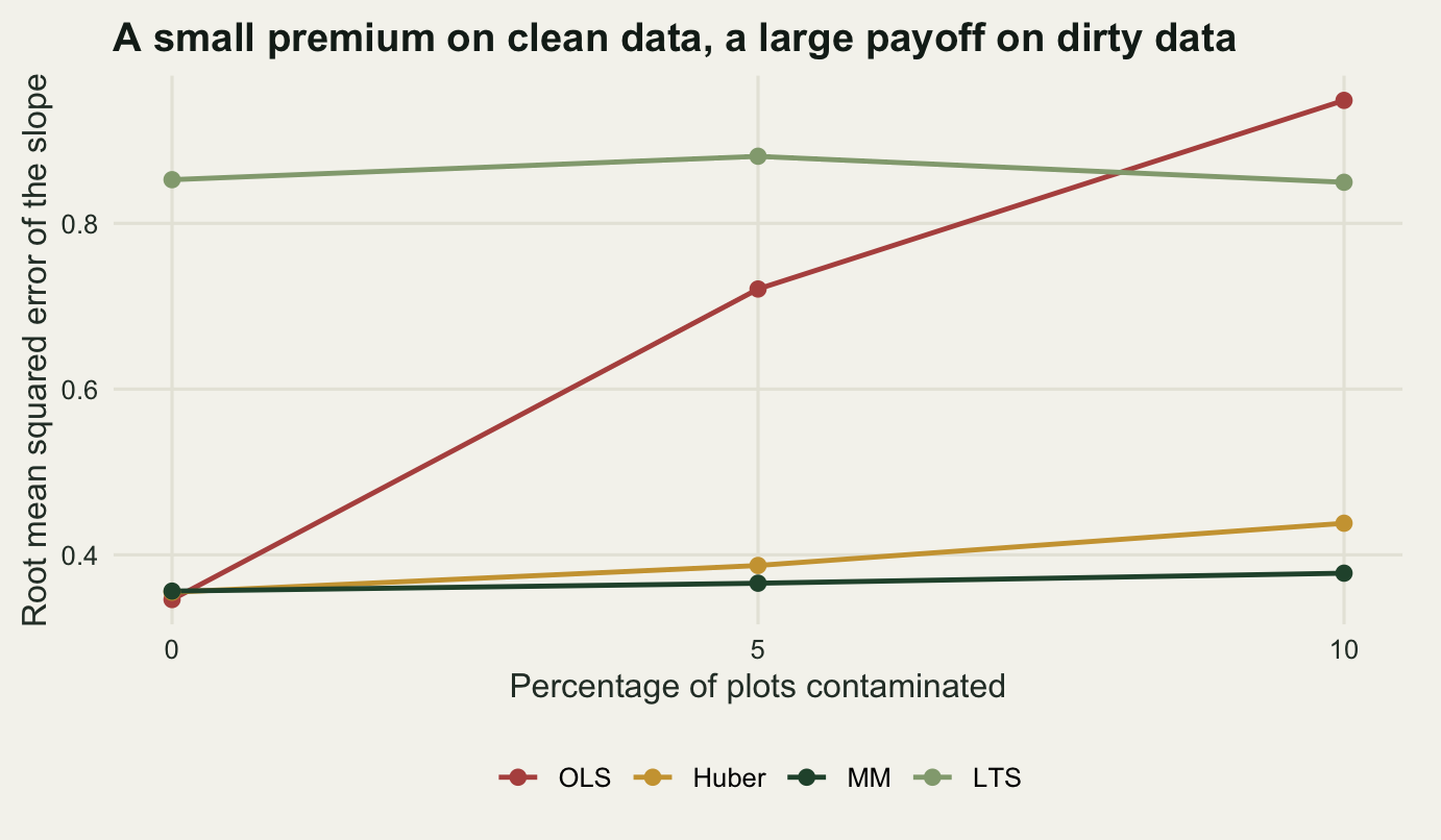
The premium buys the following. At 5 per cent contamination the root mean squared error of least squares is 0.7208 and that of the MM fit is 0.3658, a ratio of 1.97. At 10 per cent the ratio is 2.51. The MM fit’s own error barely changes across the three regimes, 0.3562, 0.3658 and 0.3779, while the least squares error goes from 0.346 to 0.9484.
The reported standard errors are honest in all three regimes. On clean data the mean reported standard error is 0.3486 against an empirical spread of 0.3461 for least squares, and 0.3586 against 0.3563 for the MM fit. Hold that result; the last section breaks it.
What robust regression does not fix
Everything so far assumed the model was right and some of the numbers were wrong. Three common situations invert that: the numbers are all correct and the model is wrong. A robust estimator handles none of them, and in two of the three it is worse than least squares while looking better. All three are items on the data exploration checklist that Zuur, Ieno and Elphick (2010) recommend working through before a model is fitted, which is the point at which they are cheapest to find.
The mast year and the mis-set counter
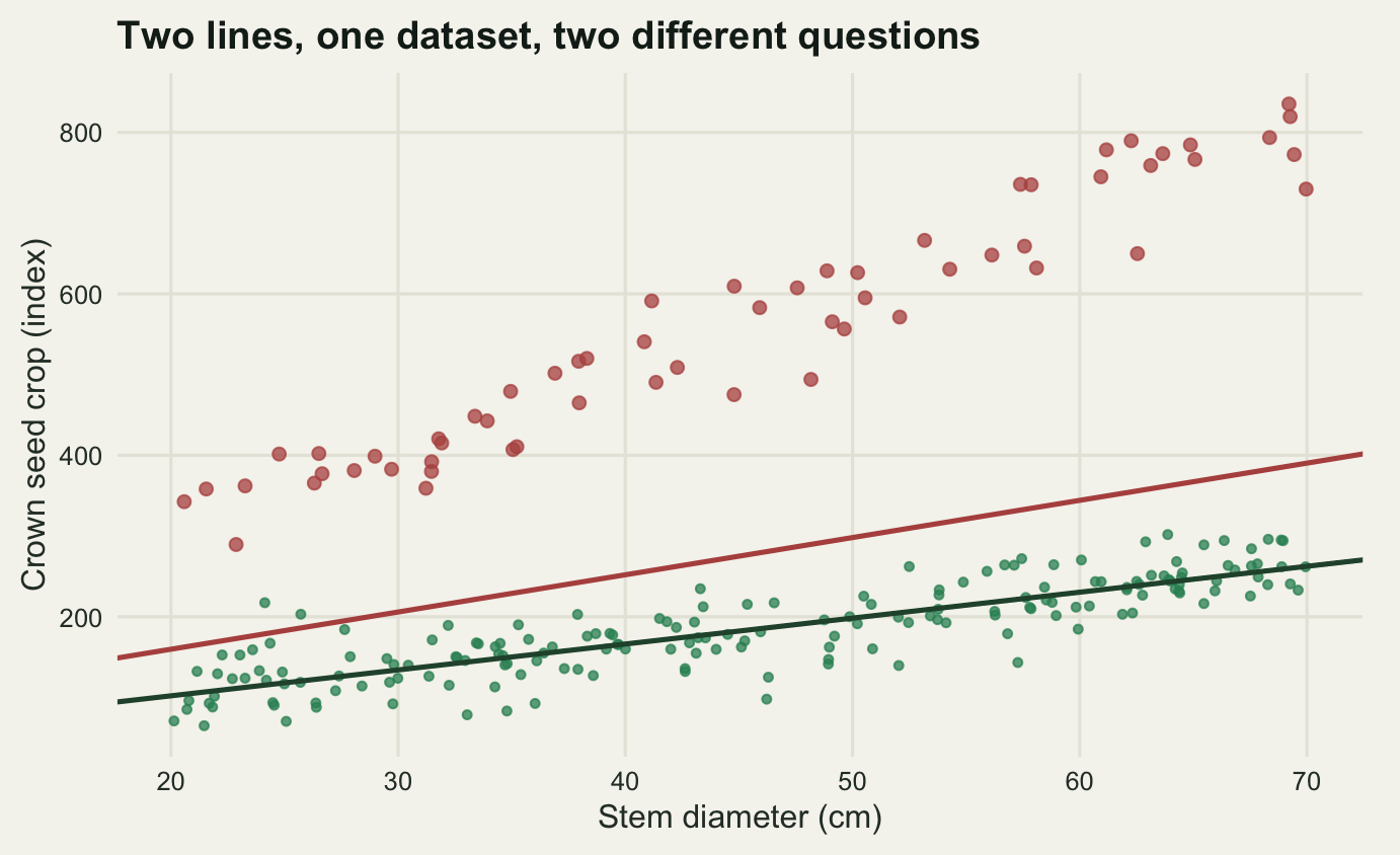
Change dataset. A seed production study: 240 tree-years of records, crown seed crop scored against stem diameter, pooled over several seasons. In 60 of those tree-years the recorded crop is far above the line, by an amount roughly proportional to what the tree would normally produce.
There are two stories for that. Either those 60 records came off a counter that had been left on a multiplier setting, or those trees were masting. The point of the section is that the two stories generate the same numbers, so the data cannot arbitrate between them, and yet they call for different answers.
n_tree <- 240
a_seed <- 40
b_seed <- 3.2
s_seed <- 30
surplus <- 2
n_mast <- 60

make_trees <- function(seed) {
  set.seed(seed)
  dbh <- runif(n_tree, 20, 70)
  base <- a_seed + b_seed * dbh
  crop <- base + rnorm(n_tree, 0, s_seed)
  which_mast <- sample.int(n_tree, n_mast)
  crop[which_mast] <- crop[which_mast] + surplus * base[which_mast] +
    rnorm(n_mast, 0, s_seed)
  list(dat = data.frame(dbh = dbh, crop = crop), mast = which_mast)
}
mixture <- 1 + surplus * n_mast / n_tree
target_bulk <- b_seed
target_mix <- mixture * b_seed

trees <- make_trees(31415)
tree_dat <- trees$dat
mast_id <- trees$mast
tree_ols <- lm(crop ~ dbh, data = tree_dat)
set.seed(202)
tree_mm <- rlm(crop ~ dbh, data = tree_dat, method = "MM", maxit = 200)

print(round(c(tree_years = n_tree, mast_years = n_mast,
              bulk_slope = target_bulk, mixture_slope = target_mix,
              ols_slope = unname(coef(tree_ols)[2]),
              ols_se = summary(tree_ols)$coefficients[2, 2],
              mm_slope = unname(coef(tree_mm)[2]),
              mm_se = summary(tree_mm)$coefficients[2, 2],
              mean_weight_mast = mean(tree_mm$w[mast_id]),
              mean_weight_rest = mean(tree_mm$w[-mast_id]),
              zero_weight_mast = sum(tree_mm$w[mast_id] < 1e-8)), 4))
tree_years mast_years bulk_slope mixture_slope
240.0000 60.0000 3.2000 4.8000
ols_slope ols_se mm_slope mm_se
4.6110 0.7407 3.2122 0.1477
mean_weight_mast mean_weight_rest zero_weight_mast
0.0009 0.9587 59.0000 The MM fit gives 3.2122 with a standard error of 0.1477, and it gets there by setting the weight of 59 of the 60 high records to exactly zero. Least squares gives 4.611 with a standard error of 0.7407, 5.02 times wider. One dataset is not enough to say what each estimator is aiming at, so run the generating process repeatedly.
n_mast_rep <- 1000
mast_ols <- mast_mm <- numeric(n_mast_rep)
for (r in seq_len(n_mast_rep)) {
  z <- make_trees(80000 + r)
  mast_ols[r] <- unname(coef(lm(crop ~ dbh, data = z$dat))[2])
  mast_mm[r] <- unname(coef(rlm(crop ~ dbh, data = z$dat,
                                method = "MM", maxit = 200))[2])
}
mast_tab <- c(mean_ols = mean(mast_ols), mc_se_ols = sd(mast_ols) / sqrt(n_mast_rep),
              mean_mm = mean(mast_mm), mc_se_mm = sd(mast_mm) / sqrt(n_mast_rep),
              ols_vs_mixture = mean(mast_ols) - target_mix,
              mm_vs_bulk = mean(mast_mm) - target_bulk,
              ols_vs_mixture_pct = 100 * (mean(mast_ols) - target_mix) / target_mix,
              mm_vs_bulk_pct = 100 * (mean(mast_mm) - target_bulk) / target_bulk,
              mm_vs_mixture_pct = 100 * (mean(mast_mm) - target_mix) / target_mix,
              ols_vs_bulk_pct = 100 * (mean(mast_ols) - target_bulk) / target_bulk)
print(round(mast_tab, 4))
mean_ols mc_se_ols mean_mm mc_se_mm
4.7715 0.0237 3.1565 0.0052
ols_vs_mixture mm_vs_bulk ols_vs_mixture_pct mm_vs_bulk_pct
-0.0285 -0.0435 -0.5947 -1.3608
mm_vs_mixture_pct ols_vs_bulk_pct
-34.2405 49.1080 Over 1000 replicates least squares averages 4.771 with a Monte Carlo standard error of 0.024, against a mixture slope of 4.8; the MM fit averages 3.156 with a Monte Carlo standard error of 0.0052, against a bulk slope of 3.2. Each sits close to its own target, off by 0.59 per cent for least squares and 1.36 per cent for the MM fit, that second residue coming from ordinary trees near the lower edge of the high records losing a little weight along with them. Each is badly wrong about the other target: the MM fit misses the mixture slope by 34.2 per cent and least squares misses the bulk slope by 49.1 per cent.
If the high records are a counter fault, the MM fit is right and least squares is inflating a biological relationship with an instrument error. If the high records are mast years, the MM fit has quietly deleted the years that produce most of the seed a forest ever sets, and the number it reports is the seed crop of an average non-mast year, which is not what a regeneration model needs. The weights are the same in both cases because the numbers are the same in both cases. No diagnostic reads intent, and the distinction lives in the field notebook, the instrument log and the phenology records, not in the residuals.
Variance that grows with the predictor
Back to the grassland. Suppose every plot is recorded correctly but the spread of biomass widens along the nitrogen gradient, which is the ordinary state of affairs in productivity data. Nothing is contaminated, so an estimator built to resist contamination has nothing to resist; the useful question is what its interval does. Two comparators go alongside it: weighted least squares given the true weights, and the sandwich standard error that White (1980) derived for exactly this situation. The version coded below divides each residual by one minus its own hat value, which is the HC3 variant of MacKinnon and White (1985); it behaves better than the original at a sample size like this one.
n_het <- 80
set.seed(6161)
x_het <- runif(n_het, 20, 60)
sd_het <- 3 + 0.022 * (x_het - 18)^2

hc3_se <- function(f) {
  Xh <- model.matrix(f)
  eh <- residuals(f)
  hh <- hatvalues(f)
  bread <- solve(crossprod(Xh))
  meat <- crossprod(Xh * (eh / (1 - hh)))
  sqrt(diag(bread %*% meat %*% bread))[2]
}

n_rep_h <- 1500
het <- matrix(NA_real_, n_rep_h, 6)
set.seed(70707)
for (r in seq_len(n_rep_h)) {
  y <- b0 + b1 * x_het + rnorm(n_het, 0, sd_het)
  d <- data.frame(nitrogen = x_het, biomass = y)
  f_o <- lm(biomass ~ nitrogen, data = d)
  f_r <- rlm(biomass ~ nitrogen, data = d, maxit = 200)
  f_w <- lm(biomass ~ nitrogen, data = d, weights = 1 / sd_het^2)
  het[r, ] <- c(coef(f_o)[2], summary(f_o)$coefficients[2, 2], hc3_se(f_o),
                coef(f_r)[2], summary(f_r)$coefficients[2, 2], coef(f_w)[2])
}
t_crit <- qt(0.975, n_het - 2)   # one multiplier for all three intervals
het_tab <- c(sd_low = min(sd_het), sd_high = max(sd_het),
             mean_ols = mean(het[, 1]), mean_rlm = mean(het[, 4]),
             mean_wls = mean(het[, 6]),
             emp_sd_ols = sd(het[, 1]), emp_sd_rlm = sd(het[, 4]),
             emp_sd_wls = sd(het[, 6]),
             reported_ols = mean(het[, 2]), reported_hc3 = mean(het[, 3]),
             reported_rlm = mean(het[, 5]),
             cover_ols = mean(abs(het[, 1] - b1) < t_crit * het[, 2]),
             cover_hc3 = mean(abs(het[, 1] - b1) < t_crit * het[, 3]),
             cover_rlm = mean(abs(het[, 4] - b1) < t_crit * het[, 5]))
print(round(het_tab, 4))
sd_low sd_high mean_ols mean_rlm mean_wls emp_sd_ols
3.2392 40.9855 4.4907 4.4925 4.4953 0.2283
emp_sd_rlm emp_sd_wls reported_ols reported_hc3 reported_rlm cover_ols
0.2043 0.1262 0.2006 0.2332 0.1489 0.9147
cover_hc3 cover_rlm
0.9433 0.8500 The residual standard deviation runs from 3.24 at the low end of the gradient to 40.99 at the high end. All three point estimates are unbiased: 4.4907 for least squares, 4.4925 for the Huber fit and 4.4953 for weighted least squares with the true weights, against a truth of 4.5. Nothing here is a bias problem.
The intervals are another matter. All three use the same multiplier, the t quantile on 78 degrees of freedom, so the coverages are comparable. The nominal ninety-five per cent interval covers the truth 91.47 per cent of the time for least squares, 94.33 per cent with a heteroscedasticity-consistent sandwich standard error, and 85.00 per cent for the Huber fit. The Huber interval is the worst of the three, and the reason is in the two columns above it: its reported standard error averages 0.1489 against an actual spread of 0.2043, so the interval is 27.1 per cent too narrow. The M-estimator’s variance formula assumes one scale for the whole dataset. Give it two and it reports the tighter one.
The estimator that belongs here is the one that models the variance. Weighted least squares with the true weights has a spread of 0.1262, or 38.2 per cent narrower than the Huber fit, and in a real analysis the weights come from a variance model rather than from omniscience: see variance structure and heteroscedasticity. A robust estimator is not a substitute for that, and the sandwich standard error is the cheap partial fix if the point estimate is all that matters.
A straight line through a curve
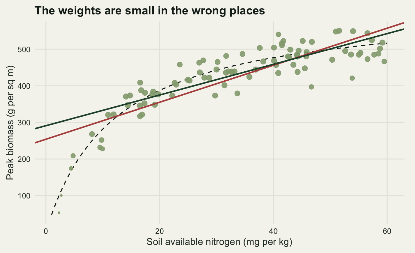
The last failure is the most ordinary. Biomass saturates with nitrogen, as it usually does past a point, and the analysis fits a straight line anyway.
n_sat <- 90
v_max <- 620
k_half <- 12
set.seed(2718)
x_sat <- runif(n_sat, 1, 60)
y_sat <- v_max * x_sat / (k_half + x_sat) + rnorm(n_sat, 0, 30)
sat_dat <- data.frame(nitrogen = x_sat, biomass = y_sat)

sat_ols <- lm(biomass ~ nitrogen, data = sat_dat)
set.seed(909)
sat_mm <- rlm(biomass ~ nitrogen, data = sat_dat, method = "MM", maxit = 200)
sat_w <- sat_mm$w
truth_at <- function(xx) v_max * xx / (k_half + xx)
pred_at <- function(f, xx) unname(predict(f, data.frame(nitrogen = xx)))
quint <- cut(x_sat, quantile(x_sat, seq(0, 1, 0.2)),
             include.lowest = TRUE, labels = FALSE)
w_rank <- suppressWarnings(cor.test(sat_w, x_sat, method = "spearman"))
curve_check <- lm(residuals(sat_mm) ~ poly(x_sat, 2))

print(round(c(ols_slope = unname(coef(sat_ols)[2]),
              ols_t = summary(sat_ols)$coefficients[2, 3],
              mm_slope = unname(coef(sat_mm)[2]),
              mm_t = summary(sat_mm)$coefficients[2, 3],
              mm_se = summary(sat_mm)$coefficients[2, 2],
              ols_se = summary(sat_ols)$coefficients[2, 2]), 4))
ols_slope ols_t mm_slope mm_t mm_se ols_se
5.0589 14.1837 4.1973 14.0696 0.2983 0.3567 print(round(c(weight_lowest_quintile = mean(sat_w[quint == 1]),
weight_rest = mean(sat_w[quint != 1]),
spearman_weight_x = unname(w_rank$estimate),
spearman_p = w_rank$p.value,
quad_t = summary(curve_check)$coefficients[3, 3],
quad_p = summary(curve_check)$coefficients[3, 4]), 5))weight_lowest_quintile weight_rest spearman_weight_x
0.72189 0.93156 0.07790
spearman_p quad_t quad_p
0.46549 -9.54754 0.00000 print(round(rbind(nitrogen = c(5, 30, 55),
truth = truth_at(c(5, 30, 55)),
ols = pred_at(sat_ols, c(5, 30, 55)),
mm = pred_at(sat_mm, c(5, 30, 55))), 2)) [,1] [,2] [,3]
nitrogen 5.00 30.00 55.00
truth 182.35 442.86 508.96
ols 279.33 405.81 532.28
mm 312.03 416.96 521.89The MM fit gives a slope of 4.197 with a t value of 14.07 and a standard error of 0.2983, against 5.059 and 0.3567 for least squares. It is the more confident of the two, and it is further from the truth where it matters most. At a nitrogen value of 5, on the steep part of the curve, the true mean biomass is 182.4; least squares predicts 279.3 and the MM fit 312, errors of 97 and 129.7 grams per square metre.
The weights do not sound the alarm. Plots in the lowest fifth of the nitrogen range carry a mean weight of 0.722 against 0.932 for the rest, so the down-weighting is concentrated where the line misses the curve, but a rank correlation between weight and nitrogen returns 0.078 with a p-value of 0.465, because the pattern is not monotone: the line misses at both ends. Regressing the MM residuals on a quadratic in nitrogen finds the curvature immediately, t of -9.55. The diagnostic that works is the old one, residuals against the predictor, and it works just as well on an M-estimator as on a least squares fit. What does not work is treating a set of small weights as evidence that the bad points have been dealt with.
What to take away
The two suspect plots in the opening notebook make three different problems. The plot clipped with the small quadrat frame, at ordinary nitrogen, is conspicuous and nearly harmless: standardised residual -8.62, slope change -0.0051, and a standard error inflated by 64.4 per cent. The sheep fold plot with nothing wrong with it is the most valuable observation in the survey, cutting the standard error by 30.6 per cent, and a rule that deletes high-leverage points would have removed it. The sheep fold plot carrying that same clipping error shows only 48 per cent of it as a residual, and moves the slope by -1.544. Residual size and damage are close to unrelated, and Cook’s distance, which multiplies the two together, is the diagnostic that ranks them correctly: 27.5 against 0.313 and 0.012.
On what to fit. The measured breakdown fractions were 1.67 per cent for least squares, 4.17 per cent for the Huber fit and 33.33 per cent for both high-breakdown estimators, when the contamination sat at extreme soil nitrogen; the same figures against contamination in the response alone were 4.17, 32.5 and no failure at all within 45 per cent. The premium for that protection on clean Gaussian data was 2.95 per cent on the standard error for the MM fit and 2.58 per cent for the Huber fit, against a payoff of 2.51 times lower root mean squared error at 10 per cent contamination. Those numbers say that fitting an MM-estimator alongside least squares should be routine, and that a disagreement between them is a finding rather than a nuisance.
The honest limit is what the disagreement means. An estimator with a fifty per cent breakdown point still gave up at 33.33 per cent here, because the contaminated plots formed a coherent cloud rather than scattered noise. Down-weighting fixed nothing when the variance grew along the gradient: the point estimate was fine, and the Huber interval covered the truth 85 per cent of the time against 91.47 per cent for the least squares interval it was supposed to improve on. It fixed nothing when a straight line was fitted through a saturating curve either, and predicted 312 where the truth was 182, further off than least squares and with a smaller standard error.
The deepest limit has no number attached because there cannot be one. When the MM fit set 59 mast records to zero weight it did the arithmetic correctly, and whether that was cleaning or vandalism depends on something the data do not contain. A weight of zero says this observation and the rest cannot both come from the same process. It does not say which process is the one you meant to study, and in ecology the extreme values are as likely to be the biology as the mistake. Irruptions, mast years, bleaching events and hundred-year floods are all points that a high-breakdown estimator will throw out without comment. The estimator can tell you how much your conclusion depends on them. Deciding whether that dependence is a weakness or the entire result is a judgement about the system, and it has to be made before the fit, written down, and defended.
References
Huber PJ 1964 The Annals of Mathematical Statistics 35(1):73-101 (10.1214/aoms/1177703732)
Cook RD 1977 Technometrics 19(1):15-18 (10.1080/00401706.1977.10489493)
Hoaglin DC, Welsch RE 1978 The American Statistician 32(1):17-22 (10.1080/00031305.1978.10479237)
Rousseeuw PJ 1984 Journal of the American Statistical Association 79(388):871-880 (10.1080/01621459.1984.10477105)
Yohai VJ 1987 The Annals of Statistics 15(2):642-656 (10.1214/aos/1176350366)
White H 1980 Econometrica 48(4):817-838 (10.2307/1912934)
MacKinnon JG, White H 1985 Journal of Econometrics 29(3):305-325 (10.1016/0304-4076(85)90158-7)
Zuur AF, Ieno EN, Elphick CS 2010 Methods in Ecology and Evolution 1(1):3-14 (10.1111/j.2041-210X.2009.00001.x)
Venables WN, Ripley BD 2002 Modern Applied Statistics with S, fourth edition (ISBN 978-0-387-95457-8)