library(ggplot2)
library(patchwork)
library(MASS)

te_paper  <- "#f5f4ee"
te_ink    <- "#16241d"
te_body   <- "#2c3a31"
te_forest <- "#275139"
te_rust   <- "#b5534e"
te_gold   <- "#c9b458"
te_line   <- "#dad9ca"

theme_datasheet <- function() {
  theme_minimal(base_size = 12) +
    theme(plot.background  = element_rect(fill = te_paper, colour = NA),
          panel.background = element_rect(fill = te_paper, colour = NA),
          panel.grid.major = element_line(colour = te_line, linewidth = 0.3),
          panel.grid.minor = element_blank(),
          text             = element_text(colour = te_body),
          plot.title       = element_text(colour = te_ink, face = "bold"),
          plot.subtitle    = element_text(colour = te_body),
          axis.text        = element_text(colour = te_body))
}Deleting outliers before the test
R
regression
hypothesis testing
simulation
statistics
ecology tutorial
Dropping points with large standardised residuals or Cook’s distance, then refitting, is a test with its own error rate. Measured in R on null regressions.
Fifty ponds, one dip net survey in each, and a regression of log tadpole density on the canopy cover over the water. The scatter looks ordinary. A few ponds sit a long way from the fitted line, and the diagnostic plots mark them: standardised residuals beyond two, or a Cook’s distance above four divided by the number of ponds. The next step in a great many analysis scripts is the same. Remove the flagged ponds, refit, and report the slope and the p value from the second fit, with a sentence in the methods saying that outliers were excluded.
The step reads like housekeeping. It is a decision made with the response values, before the test that uses the same response values, and the test at the end does not know the decision was made. Its error rate is therefore not the nominal rate of the t test on the slope, and nothing in the output says what it is.
Robust regression for ecological outliers makes the argument against the reflex and shows it on single plots: finding the points far from the fitted line and dropping them is circular, because the line was fitted with those points in it. That post then builds leverage, standardised residuals and Cook’s distance by hand, measures the breakdown point of M-estimators and the efficiency they give up on clean data, and never runs the delete and refit rule to see what it does to a test. That is the number measured here, on data that contain no outliers at all and no slope, where every rejection is a false one. Pretesting variances before a t test measured a different data dependent choice made before a test, a variance check that picks which test to run; here nothing picks the test, the data themselves are edited.
The post runs four rules on the same simulated surveys at three sample sizes: delete once on the standardised residual, delete once on Cook’s distance, delete on the standardised residual until nothing is flagged, and delete only if the first fit was not significant. It then explains the inflation, repeats the whole thing with heavy tailed errors, where outlier rules are supposed to earn their place, and ends with the robust fit as the alternative.
The rule, run on one survey
The generating model has no slope. Canopy cover is standardised, log density is pure noise around a constant, and the errors are normal with the same variance everywhere, so every assumption of the ordinary regression test holds exactly. The two flags are the ones R returns: rstandard() gives the internally studentised residual, the raw residual divided by the residual standard error times the square root of one minus the hat value, and cooks.distance() gives Cook’s distance. The cut-offs are the rule of thumb values, an absolute standardised residual above 2 and a Cook’s distance above 4 divided by the sample size.
alpha_lev <- 0.05
rs_cut    <- 2                       # absolute standardised residual
cook_mult <- 4                       # Cook's distance above cook_mult / n
n_ponds   <- 50                      # the worked survey

set.seed(2908)
ponds <- data.frame(canopy = rnorm(n_ponds))
ponds$log_dens <- 1.5 + rnorm(n_ponds)    # no slope: the null is true

fit_all  <- lm(log_dens ~ canopy, data = ponds)
rs_obs   <- rstandard(fit_all)
cook_obs <- cooks.distance(fit_all)
flag_rs   <- abs(rs_obs) > rs_cut
flag_cook <- cook_obs > cook_mult / n_ponds
fit_rs   <- lm(log_dens ~ canopy, data = ponds[!flag_rs, ])
fit_cook <- lm(log_dens ~ canopy, data = ponds[!flag_cook, ])
row_of <- function(f) summary(f)$coefficients["canopy", ]
ex_tab <- rbind(all = row_of(fit_all), rs = row_of(fit_rs), cook = row_of(fit_cook))
ex_df  <- c(df.residual(fit_all), df.residual(fit_rs), df.residual(fit_cook))
round(cbind(ex_tab, df = ex_df), 4)
Estimate Std. Error t value Pr(>|t|) df
all -0.3886 0.1692 -2.2969 0.0260 48
rs -0.3353 0.1581 -2.1211 0.0396 44
cook -0.3685 0.1548 -2.3801 0.0219 42In this survey 4 ponds have an absolute standardised residual above 2 and 6 have a Cook’s distance above 0.08. On all 50 ponds the slope is -0.389 with a standard error of 0.169 and a p value of 0.026. With the residual flags removed it is -0.335, standard error 0.158, p value 0.040, on 44 residual degrees of freedom; with the Cook flags removed it is -0.369, standard error 0.155, p value 0.022, on 42. This survey was drawn with no slope, so the first fit is already one of the one in twenty false positives, and the two rules move its p value in opposite directions. The refit is an ordinary lm() on fewer rows, so its degrees of freedom are those of the reduced sample.
One survey says nothing about a rate. Thousands of surveys do, and lm() inside a loop is slow, so the simulation below fits every survey at once. For a single predictor the least squares fit, the hat values, the standardised residuals and Cook’s distance are all sums over the retained rows, and a 0/1 matrix of retained rows turns thousands of fits into a handful of column sums. That is a claim to check against R’s own functions before any rate is computed from it.
# X, Y: n by R matrices (one column per survey); W: 1 = row kept, 0 = deleted
fit_mask <- function(X, Y, W) {
  n <- nrow(X); m <- colSums(W)
  xbar <- colSums(W * X) / m; ybar <- colSums(W * Y) / m
  sxx  <- colSums(W * X^2) - m * xbar^2
  b    <- (colSums(W * X * Y) - m * xbar * ybar) / sxx
  a    <- ybar - b * xbar
  E    <- Y - rep(a, each = n) - X * rep(b, each = n)
  s2   <- colSums(W * E^2) / (m - 2)
  H    <- W * (rep(1 / m, each = n) + (X - rep(xbar, each = n))^2 / rep(sxx, each = n))
  RS   <- W * E / sqrt(rep(s2, each = n) * (1 - H))
  CD   <- RS^2 * H / (2 * (1 - H))
  se   <- sqrt(s2 / sxx)
  list(b = b, se = se, p = 2 * pt(-abs(b / se), m - 2), m = m, rs = RS, cook = CD)
}
one <- function(v) matrix(v, ncol = 1)
chk_all <- fit_mask(one(ponds$canopy), one(ponds$log_dens), one(rep(1, n_ponds)))
chk_rs  <- fit_mask(one(ponds$canopy), one(ponds$log_dens), one(as.numeric(!flag_rs)))
id_gap <- max(abs(c(chk_all$rs - rs_obs, chk_all$cook - cook_obs,
                    chk_rs$b - ex_tab["rs", 1], chk_rs$se - ex_tab["rs", 2],
                    chk_rs$p - ex_tab["rs", 4])))
# adding a real slope changes no residual, so no flag and no pivotal t changes
slope_add <- 0.7
ponds$shifted <- ponds$log_dens + slope_add * ponds$canopy
fit_shift <- lm(shifted ~ canopy, data = ponds)
shift_gap <- max(abs(c(rstandard(fit_shift) - rs_obs,
  (coef(lm(shifted ~ canopy, data = ponds[!flag_rs, ]))[2] - slope_add) - ex_tab["rs", 1])))
The matrix version agrees with rstandard(), cooks.distance() and the refitted lm() to 8.9e-16, which is rounding error. A second check is worth making once, because it saves a whole simulation. Adding a real slope of 0.7 to the same survey changes the standardised residuals by 1.8e-15: the same ponds are flagged, and the refitted estimate minus the true slope is the same number as before. So for the rules that act on residuals alone (once, on Cook’s distance, and until clean) the rate at which a rule rejects a true null slope of zero is exactly the rate at which its 95 per cent interval misses a true slope of any size, and the type I rates below are also coverage failures. The conditional rule is the exception: whether it deletes depends on the p value for a zero slope, which does change when a slope is added, and its coverage is measured separately below.
Deleting once doubles the false positive rate
Each simulated survey draws its own canopy values and its own noise, with no slope, at 20, 50 and 200 ponds. Every rule is applied to the same surveys. The replicate count was fixed before any rate was computed.
n_grid <- c(20, 50, 200)
n_rep  <- 10000
max_iter <- 200

run_rules <- function(n, n_rep, err_draw) {
  X <- matrix(rnorm(n * n_rep), n)
  Y <- matrix(err_draw(n * n_rep), n)
  W <- matrix(1, n, n_rep)
  f0 <- fit_mask(X, Y, W)
  W_rs   <- W * (abs(f0$rs) <= rs_cut)
  W_cook <- W * (f0$cook <= cook_mult / n)
  f_rs <- fit_mask(X, Y, W_rs); f_cook <- fit_mask(X, Y, W_cook)
  W_it <- W; n_iter <- 0; traj <- NULL
  repeat {                                  # delete until nothing is flagged
    f_it <- fit_mask(X, Y, W_it); n_iter <- n_iter + 1
    traj <- rbind(traj, c(round = n_iter - 1, rate = mean(f_it$p < alpha_lev),
                          removed = mean(1 - f_it$m / n)))
    new_flag <- W_it * (abs(f_it$rs) > rs_cut)
    if (!any(new_flag > 0) || n_iter >= max_iter) break
    W_it <- W_it - new_flag
  }
  p_cond <- ifelse(f0$p > alpha_lev, f_rs$p, f0$p)
  r_flag <- W * (pf(f0$cook, 2, n - 2) > 0.5)      # the flag influence.measures() uses
  list(n = n, f0 = f0, f_rs = f_rs, X = X, Y = Y,
       rate = c(none = mean(f0$p < alpha_lev), rs_once = mean(f_rs$p < alpha_lev),
                cook_once = mean(f_cook$p < alpha_lev), rs_iter = mean(f_it$p < alpha_lev),
                cond = mean(p_cond < alpha_lev)),
       removed = c(none = 0, rs_once = mean(1 - f_rs$m / n), cook_once = mean(1 - f_cook$m / n),
                   rs_iter = mean(1 - f_it$m / n), cond = mean((f0$p > alpha_lev) * (1 - f_rs$m / n))),
       traj = data.frame(n = n, traj), n_iter = n_iter, min_kept = min(f_it$m), r_flag = mean(colSums(r_flag) > 0),
       cook_any = mean(colSums(W - W_cook) > 0), cook_pts = mean(colSums(W - W_cook)))
}
rule_lev <- c("no deletion", "residual, once", "Cook, once", "residual, until clean",
              "residual, if not significant")
set.seed(7431)
norm_runs <- lapply(n_grid, run_rules, n_rep = n_rep, err_draw = rnorm)
tab_rules <- function(runs) do.call(rbind, lapply(runs, function(r)
  data.frame(n = r$n, rule = factor(rule_lev, levels = rule_lev),
             rate = unname(r$rate), removed = unname(r$removed))))
norm_tab <- tab_rules(norm_runs)
norm_tab$mcse <- sqrt(norm_tab$rate * (1 - norm_tab$rate) / n_rep)
rt_at <- function(tab, n, k) tab$rate[tab$n == n & tab$rule == rule_lev[k]]
rm_at <- function(tab, n, k) tab$removed[tab$n == n & tab$rule == rule_lev[k]]
mcse_top <- max(norm_tab$mcse)
iter_used <- vapply(norm_runs, function(r) r$n_iter, 0)
min_kept  <- vapply(norm_runs, function(r) r$min_kept, 0)
r_flag50  <- norm_runs[[2]]$r_flag
cook_any50 <- norm_runs[[2]]$cook_any; cook_pts50 <- norm_runs[[2]]$cook_pts
# every criterion influence.measures() marks (dfbetas, dffit, cov.r, cook.d, hat), null surveys of 50 ponds
n_im <- 2000
set.seed(3361)
im_rows <- replicate(n_im, {
  x <- rnorm(n_ponds); y <- rnorm(n_ponds)
  sum(rowSums(influence.measures(lm(y ~ x))$is.inf) > 0)
})
im_any50 <- mean(im_rows > 0); im_pts50 <- mean(im_rows)
rise_20_200 <- vapply(2:5, function(k) rt_at(norm_tab, 200, k) - rt_at(norm_tab, 20, k), 0)
mcse_diff <- sqrt(2) * mcse_top
Without deletion the slope test rejects 5.2, 5.0 and 5.1 per cent of the time at 20, 50 and 200 ponds, which is the exact test doing its job. Deleting the ponds with an absolute standardised residual above 2 once and refitting gives 10.7, 10.9 and 11.0 per cent, while removing 4.4 per cent of perfectly normal data at 50 ponds. The Cook rule gives 9.4, 9.6 and 9.9 per cent. The largest Monte Carlo standard error in the whole table is 0.44 percentage points.
The rates do not fall as the survey grows. From 20 to 200 ponds the residual, Cook and conditional rules move by +0.4, +0.5 and +0.5 percentage points, against a Monte Carlo standard error for a difference of at most 0.63 points, so they hold level; the rule that deletes until clean, measured below, climbs by 9.3 points. More data does not dilute the problem. One round of residual deletion removes 4.2 per cent of the data at 20 ponds and 4.5 per cent at 200, so the share of the sample that is edited stays put while the sample grows.
Cook’s distance is not the only threshold in circulation. R’s own influence.measures() marks a point as influential when its Cook’s distance exceeds the median of an F distribution with 2 and n minus 2 degrees of freedom, which is close to Cook’s own suggestion of reading the distance against F quantiles. At 50 ponds that cut-off is 0.70, against 0.08 for 4 divided by n. On the Cook column alone at least one pond is flagged in 0.69 per cent of null surveys, against 97.4 per cent for the 4 divided by n cut-off, which marks 2.72 ponds per survey on average. The F median is the far more lenient bar, and 4 divided by n is the one that removes data. The asterisks in summary(influence.measures()) are a different matter: they also mark hat values, dffits, dfbetas and covariance ratios, and in 2000 null surveys of 50 ponds some row was marked in 99.9 per cent of them, 4.54 rows per survey on average. A script that deletes every marked row deletes in nearly every survey.
ggplot(norm_tab, aes(factor(n), 100 * rate, colour = rule, linetype = rule, group = rule)) +
  geom_hline(yintercept = 100 * alpha_lev, colour = te_body, linetype = "dashed", linewidth = 0.5) +
  geom_errorbar(aes(ymin = 100 * (rate - 2 * mcse), ymax = 100 * (rate + 2 * mcse)),
                width = 0.12, linewidth = 0.4, linetype = "solid") +
  geom_line(linewidth = 0.9) + geom_point(size = 2.2) +
  scale_colour_manual(values = c(te_forest, te_gold, te_gold, te_rust, te_ink), name = NULL) +
  scale_linetype_manual(values = c("solid", "solid", "22", "solid", "solid"), name = NULL) +
  scale_y_continuous(limits = c(0, NA)) +
  guides(colour = guide_legend(nrow = 2)) +
  labs(x = "ponds in the survey", y = "rejection rate under the null (per cent)",
       title = "Deleting outliers from clean data",
       subtitle = "dashed line: the nominal five per cent; bars: two Monte Carlo standard errors") +
  theme_datasheet() + theme(legend.position = "bottom")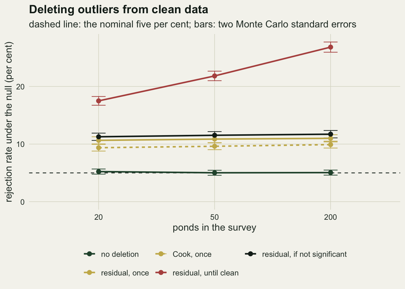
The standard error shrinks and the slope does not
The obvious explanation is the residual standard error. Removing every residual beyond two standard deviations leaves a truncated normal sample, whose standard deviation is smaller than that of the errors that generated the slope. The standard error is computed from the truncated residuals, so it is too small, and the t statistic is too large. That argument gives a number, and the number can be compared with the measurement.
trunc_sd <- sqrt(1 - 2 * rs_cut * dnorm(rs_cut) / (2 * pnorm(rs_cut) - 1))
naive_rate <- 2 * pnorm(-qnorm(1 - alpha_lev / 2) * trunc_sd)
mech <- do.call(rbind, lapply(norm_runs, function(r)
  data.frame(n = r$n,
             sd_b_all = sd(r$f0$b), se_all = sqrt(mean(r$f0$se^2)),
             sd_b_rs = sd(r$f_rs$b), se_rs = sqrt(mean(r$f_rs$se^2)),
             sd_change = sd(r$f_rs$b - r$f0$b),
             push = cov(r$f_rs$b - r$f0$b, r$f0$b) / var(r$f0$b))))
mech$ratio_rs  <- mech$sd_b_rs / mech$se_rs
mech$ratio_all <- mech$sd_b_all / mech$se_all
m50 <- mech[mech$n == 50, ]
implied50 <- 2 * pnorm(-qnorm(1 - alpha_lev / 2) / m50$ratio_rs)
df50_rs <- mean(norm_runs[[2]]$f_rs$m) - 2
implied50_t <- 2 * pt(-qt(1 - alpha_lev / 2, df50_rs) / m50$ratio_rs, df50_rs)
# control: delete the same number of ponds from each survey, chosen at random
r50 <- norm_runs[[2]]; n50 <- nrow(r50$X)
k_del <- n50 - r50$f_rs$m
set.seed(1187)
rank_mat <- apply(matrix(runif(length(r50$X)), n50), 2, rank)
W_rand <- 1 * (rank_mat > rep(k_del, each = n50))
f_rand <- fit_mask(r50$X, r50$Y, W_rand)
sd_b_rand <- sd(f_rand$b); rate_rand <- mean(f_rand$p < alpha_lev)
rand_share <- (sd_b_rand^2 - m50$sd_b_all^2) / (m50$sd_b_rs^2 - m50$sd_b_all^2)
mcse_rand <- sqrt(rate_rand * (1 - rate_rand) / n_rep)
p_hist <- rbind(data.frame(fit = "all ponds", p = norm_runs[[2]]$f0$p),
                data.frame(fit = "after deleting |residual| > 2", p = norm_runs[[2]]$f_rs$p))
p_hist$fit <- factor(p_hist$fit, levels = c("all ponds", "after deleting |residual| > 2"))
below01 <- c(mean(norm_runs[[2]]$f0$p < 0.01), mean(norm_runs[[2]]$f_rs$p < 0.01))
A normal distribution cut at plus and minus 2 has a standard deviation of 0.880, and a t statistic inflated by the reciprocal of that would reject 8.5 per cent of the time. The measured rate at 50 ponds is 10.9 per cent, so the shrinking standard error is only part of the story.
The other part is the slope. At 50 ponds the standard deviation of the slope across surveys is 0.1455 on all ponds and 0.1605 after deletion: the estimate gets noisier, not steadier. Its root mean square standard error moves the other way, from 0.1460 to 0.1319. The ratio of true spread to reported standard error is 0.997 without deletion and 1.217 after it, and a normal statistic inflated by that ratio rejects 10.7 per cent of the time on a normal reference (10.5 per cent on a t reference with the average reduced degrees of freedom), which is close to the measured rate.
Losing a few ponds explains only a small part of the extra spread. Deleting the same number of ponds from each survey at random leaves the slope with a standard deviation of 0.1496, which accounts for 26 per cent of the extra variance that residual deletion adds, and that test rejects 5.0 per cent of the time (Monte Carlo standard error 0.22 points), because random deletion does not select on the response. What the flagged ponds have in common is a large residual, and removing a pond moves the slope by an amount proportional to its residual times its distance from the mean canopy cover. Each deletion is a large kick to the slope. A natural guess is that the kick pushes the line further in the direction the first fit already leaned, but the measurement does not support it: regressing the change in slope on the first slope gives a coefficient of -0.002 at 50 ponds, 0.003 at 20 and 0.012 at 200, all near zero. The kick is noise added on top of the first estimate, with a standard deviation of 0.0682 at 50 ponds, and the refitted standard error, computed from the residuals that survived, has no term for it.
p_left <- ggplot(p_hist, aes(p, fill = fit)) +
  geom_histogram(breaks = seq(0, 1, by = 0.05), colour = te_paper, linewidth = 0.2) +
  facet_wrap(~ fit, ncol = 1) +
  scale_fill_manual(values = c(te_forest, te_rust), guide = "none") +
  labs(x = "p value for the slope", y = "surveys", title = "Null p values",
       subtitle = "a valid test gives a flat histogram") +
  theme_datasheet()

mech_long <- rbind(
  data.frame(n = mech$n, fit = "all ponds", what = "spread of the slope", value = mech$sd_b_all),
  data.frame(n = mech$n, fit = "all ponds", what = "reported standard error", value = mech$se_all),
  data.frame(n = mech$n, fit = "after deletion", what = "spread of the slope", value = mech$sd_b_rs),
  data.frame(n = mech$n, fit = "after deletion", what = "reported standard error", value = mech$se_rs))
mech_long$fit <- factor(mech_long$fit, levels = c("all ponds", "after deletion"))
mech_long$scaled <- mech_long$value / rep(mech$sd_b_all, 4)
p_right <- ggplot(mech_long[mech_long$n == 50, ], aes(fit, scaled, fill = what)) +
  geom_col(position = position_dodge(width = 0.7), width = 0.6, colour = te_paper, linewidth = 0.3) +
  geom_hline(yintercept = 1, colour = te_body, linetype = "dashed", linewidth = 0.5) +
  scale_fill_manual(values = c(te_gold, te_forest), name = NULL) +
  guides(fill = guide_legend(nrow = 2)) +
  labs(x = NULL, y = "relative to the spread on all ponds", title = "Spread against reported error",
       subtitle = "50 ponds") +
  theme_datasheet() + theme(legend.position = "bottom")

p_left + p_right + plot_annotation(theme = theme_datasheet())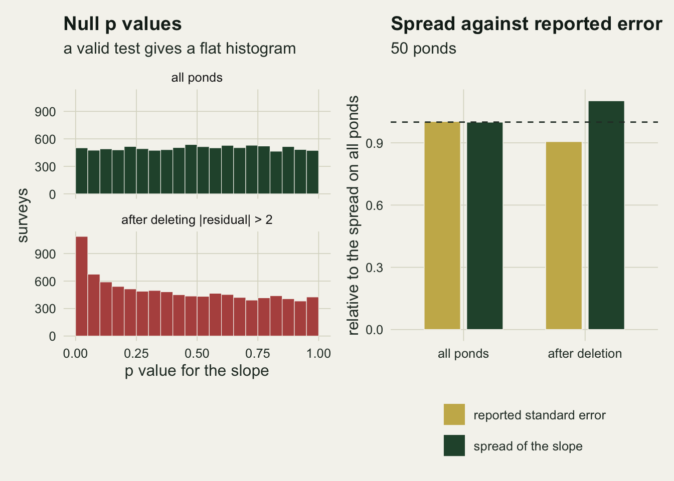
The left panel shows where the extra rejections come from. With all ponds, 1.0 per cent of null p values fall below 0.01; after one round of deletion 3.2 per cent do. The histogram after deletion is piled up against zero, which is what a test that overstates its own precision looks like.
Until clean, or only when it helps
Two versions of the rule are worse. The first repeats the deletion: refit, recompute the standardised residuals, and delete again while anything is flagged. Because each refit shrinks the residual standard error, some of the remaining residuals cross the threshold, and the rule keeps finding new outliers in data that never had any. The second is the version that is rarely written down: delete only when the first fit is not significant, and keep the first fit when it already is.
traj_tab <- do.call(rbind, lapply(norm_runs, function(r) r$traj))
traj_gap <- max(vapply(norm_runs, function(r)
  abs(r$traj$rate[r$traj$round == 1] - r$rate[["rs_once"]]), 0))
round_at <- function(n, k) traj_tab[traj_tab$n == n & traj_tab$round == k, ]
cond_extra <- vapply(norm_runs, function(r) mean(r$f0$p > alpha_lev & r$f_rs$p < alpha_lev), 0)
# coverage of the conditional rule when the true slope is not zero (50 ponds): residuals and the
# pivotal t are unchanged, but the trigger is the p value for a zero slope on the shifted data
slope_grid <- c(0.2, 0.7)
cond_miss <- vapply(slope_grid, function(b) {
  r <- norm_runs[[2]]
  p_zero <- 2 * pt(-abs((r$f0$b + b) / r$f0$se), r$f0$m - 2)
  mean(ifelse(p_zero > alpha_lev, r$f_rs$p, r$f0$p) < alpha_lev)
}, 0)
Deleting until nothing is flagged rejects a true null 17.5 per cent of the time at 20 ponds, 21.8 per cent at 50 and 26.8 per cent at 200, and it removes 7.9, 11.1 and 13.4 per cent of the data on average. This rule does get worse with sample size. It stopped on its own in every survey, after at most 10, 18 and 26 rounds of deletion at 20, 50 and 200 ponds, and no survey was cut below 10 ponds. The first round of the loop is the single deletion rule, and its rate is the same as the one above (largest difference 0.0000). At 200 ponds the second round takes the rate to 16.3 per cent with 7.7 per cent of the data gone, and the fifth to 23.8 per cent with 11.8 per cent gone.
Deleting only after a non-significant first fit rejects 11.3, 11.5 and 11.7 per cent of the time. That is slightly higher than deleting in every survey, at each sample size, even though it deletes in fewer surveys. The first fit’s rejections are kept, and the deletion adds the surveys that were not significant before and are after: 6.5 per cent of all surveys at 50 ponds. A rule that deletes in every survey also loses some rejections the first fit had, and the conditional rule never gives any back. Its coverage is not the same number: with a true slope of 0.2 at 50 ponds its 95 per cent interval misses the true slope in 7.9 per cent of surveys, and with a slope of 0.7 in 5.0 per cent, because a steep slope is significant before any deletion and the first fit is kept.
traj_plot <- traj_tab[traj_tab$round <= 12, ]
traj_plot$ponds <- factor(paste(traj_plot$n, "ponds"), levels = paste(n_grid, "ponds"))
p_tr_rate <- ggplot(traj_plot, aes(round, 100 * rate, colour = ponds)) +
  geom_hline(yintercept = 100 * alpha_lev, colour = te_body, linetype = "dashed", linewidth = 0.5) +
  geom_line(linewidth = 0.9) + geom_point(size = 1.8) +
  scale_colour_manual(values = c(te_gold, te_forest, te_rust), name = NULL) +
  scale_x_continuous(breaks = seq(0, 12, by = 2)) +
  scale_y_continuous(limits = c(0, NA)) +
  labs(x = "rounds of deletion", y = "rejection rate under the null (per cent)",
       title = "Type I error", subtitle = "round 0: no deletion") +
  theme_datasheet() + theme(legend.position = "bottom")
p_tr_rm <- ggplot(traj_plot, aes(round, 100 * removed, colour = ponds)) +
  geom_line(linewidth = 0.9) + geom_point(size = 1.8) +
  scale_colour_manual(values = c(te_gold, te_forest, te_rust), name = NULL) +
  scale_x_continuous(breaks = seq(0, 12, by = 2)) +
  scale_y_continuous(limits = c(0, NA)) +
  labs(x = "rounds of deletion", y = "per cent of the data removed",
       title = "Data removed", subtitle = "averaged over all surveys") +
  theme_datasheet() + theme(legend.position = "bottom")
p_tr_rate + p_tr_rm + plot_layout(guides = "collect") +
  plot_annotation(theme = theme_datasheet() + theme(legend.position = "bottom"))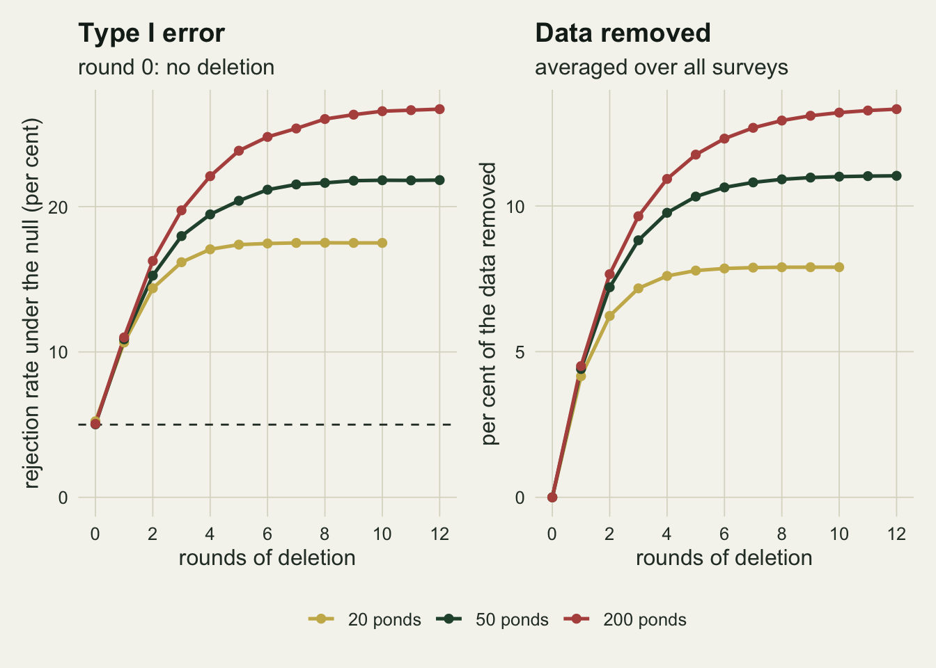
Heavy tails, the case the rule is meant for
The defence of the rule is that real data are not normal. Ecological residuals often have heavier tails than a normal distribution, and a few extreme values in a small survey can move a least squares slope a long way. So the fair test is on errors from a t distribution with 3 degrees of freedom, heavy tailed but with finite variance, where the ordinary test is no longer exact. The baseline matters here: the inflation has to be read against what the undeleted test does on the same errors, not against five per cent.
t_df <- 3
set.seed(5217)
heavy_runs <- lapply(n_grid, run_rules, n_rep = n_rep,
                     err_draw = function(k) rt(k, t_df))
heavy_tab <- tab_rules(heavy_runs)
heavy_tab$mcse <- sqrt(heavy_tab$rate * (1 - heavy_tab$rate) / n_rep)
eff_gain50 <- sd(heavy_runs[[2]]$f_rs$b) / sd(heavy_runs[[2]]$f0$b)
se_gain50 <- sqrt(mean(heavy_runs[[2]]$f_rs$se^2) / mean(heavy_runs[[2]]$f0$se^2))

n_rlm <- 2000
rlm_reject <- function(err_draw) {
  x <- rnorm(n_ponds); y <- err_draw(n_ponds)
  tv <- summary(rlm(y ~ x, maxit = 50))$coefficients["x", "t value"]
  abs(tv) > qt(1 - alpha_lev / 2, n_ponds - 2)
}
set.seed(6044)
rlm_norm  <- mean(replicate(n_rlm, rlm_reject(rnorm)))
rlm_heavy <- mean(replicate(n_rlm, rlm_reject(function(k) rt(k, t_df))))
mcse_rlm  <- sqrt(alpha_lev * (1 - alpha_lev) / n_rlm)
With t errors and no deletion the test rejects 5.6, 5.1 and 5.2 per cent of the time: least squares loses efficiency on heavy tails, but its level stays within a point of nominal. One round of residual deletion gives 9.5, 8.5 and 8.0 per cent, the Cook rule 7.9, 7.2 and 6.4 per cent, deleting until clean 19.2, 24.2 and 29.1 per cent, and the conditional rule 11.2, 10.6 and 10.4 per cent.
Here the single deletion rules do ease off as the survey grows, which they did not do on normal data; with genuinely heavy tails some of what they remove really is the tail the least squares fit should not have trusted, though that reading was not measured separately. They stay above the undeleted baseline at every size measured; whether they reach it at larger surveys was not run. Deleting until clean goes the other way and climbs with sample size, as it did on normal data.
The deletion is not useless here. At 50 ponds one round of it cuts the spread of the slope to 0.77 of its value without deletion, so the estimate itself is better. The test built on it is still wrong, because the reported standard error falls further, to 0.68 of its value.
The alternative that gets the efficiency without editing the data is to downweight rather than delete, which is what robust regression does. A Huber M-estimate from MASS::rlm(), with its t value compared against a t distribution on n minus 2 degrees of freedom, rejected 4.2 per cent of 2000 null surveys of 50 ponds with normal errors and 4.9 per cent with t errors, both within two Monte Carlo standard errors of five per cent (one standard error is 0.5 points).
bar_lev <- c(rule_lev, "Huber rlm, no deletion")
heavy_bars <- rbind(
  data.frame(errors = "normal errors", rule = rule_lev, rate = norm_tab$rate[norm_tab$n == 50]),
  data.frame(errors = "t errors, 3 df", rule = rule_lev, rate = heavy_tab$rate[heavy_tab$n == 50]),
  data.frame(errors = c("normal errors", "t errors, 3 df"), rule = bar_lev[6],
             rate = c(rlm_norm, rlm_heavy)))
heavy_bars$rule <- factor(heavy_bars$rule, levels = rev(bar_lev))
ggplot(heavy_bars, aes(100 * rate, rule, fill = errors)) +
  geom_col(position = position_dodge(width = 0.75), width = 0.7, colour = te_paper, linewidth = 0.3) +
  geom_vline(xintercept = 100 * alpha_lev, colour = te_body, linetype = "dashed", linewidth = 0.5) +
  scale_fill_manual(values = c(te_forest, te_rust), name = NULL) +
  labs(x = "rejection rate under the null (per cent)", y = NULL,
       title = "Heavy tails do not rescue the rule",
       subtitle = "50 ponds; dashed line: the nominal five per cent") +
  theme_datasheet() + theme(legend.position = "bottom")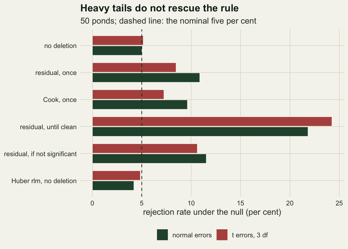
What to report
If points were deleted, report the fit with all points as well, in the main text rather than a supplement. Simmons, Nelson and Simonsohn (2011) list this among their requirements for authors: when observations are eliminated, the results with them included are reported too. The exclusion is a choice made after seeing the data, and a reader cannot correct for a choice that is not shown. Fraser and colleagues (2018) surveyed ecologists and evolutionary biologists and found that large shares admitted to leaving out non-significant results and to collecting more data after checking for significance, so the analytic flexibility that study described is not confined to psychology.
Give the rule, the threshold and the number of points it removed, and say whether it was fixed before the data were seen. The difference between deleting once and deleting only after a non-significant fit is invisible in a results table and it changes the error rate.
Do not delete because a point is far from the line. Delete because there is a record that it is wrong: a mislabelled sample, a broken net, a data entry error that the field sheet can confirm. That is a statement about the observation, and it holds whether or not the point is flagged. A diagnostic flag without such a record is a statement about the model, and the answer to it is a different model.
When the tails are heavy, fit a model that expects heavy tails, with a robust fit or a t distributed error, and report it as the primary analysis with the least squares fit beside it. Bakker and Wicherts (2014) reached the same recommendation for two group comparisons, where removing values beyond a z threshold inflated the type I error of the t test, and they recommended a rank based test or the Yuen-Welch test on trimmed means in place of removal.
Honest limits
Everything here is a single predictor with a symmetric error distribution and no true outliers. With a contaminated sample, where some points really do come from a different process, deleting them can remove bias that no test correction fixes, and the trade between that bias and the inflated error rate was not measured. The null case isolates the cost of the rule; it cannot say when the cost is worth paying.
The predictor is drawn from a normal distribution in every survey, so high leverage points occur only by chance. A design with a few extreme predictor values, such as a gradient with most sites at one end, changes which points the Cook rule flags, and the Cook rates above should not be carried to such designs without rerunning the code.
The cut-offs are fixed at the two rule of thumb values. Bakker and Wicherts found the inflation is worst when the threshold itself is chosen after looking at the results, and that version, trying 2, 2.5 and 3 and keeping the one that works, was not simulated. Its rate is bounded below by the conditional rule measured here.
The t distribution with 3 degrees of freedom is one kind of heavy tail. Skewed errors, which are more common in ecological responses such as biomass, put the flagged points mostly on one side of the line, and the deletion would then be expected to shift the intercept as well as distort the test; that case was not run. The M-estimator comparison uses one estimator at one sample size, with a Monte Carlo error large enough that it shows the level is near nominal, not that it is exactly so. Robust regression for ecological outliers measures what that estimator costs in efficiency and where it breaks.
References
Cook RD 1977 Technometrics 19(1):15-18 (10.1080/00401706.1977.10489493)
Simmons JP, Nelson LD, Simonsohn U 2011 Psychological Science 22(11):1359-1366 (10.1177/0956797611417632)
Bakker M, Wicherts JM 2014 Psychological Methods 19(3):409-427 (10.1037/met0000014)
Fraser H, Parker T, Nakagawa S, Barnett A, Fidler F 2018 PLoS ONE 13(7):e0200303 (10.1371/journal.pone.0200303)