library(ggplot2)

te_pal <- list(forest = "#275139", green = "#2f8f63", sage = "#93a87f",
               clay = "#b5534e", gold = "#cda23f", line = "#dad9ca",
               ink = "#16241d", paper = "#f5f4ee")

theme_te <- function() {
  theme_minimal(base_size = 12) +
    theme(panel.grid.minor = element_blank(),
          panel.grid.major = element_line(colour = "#e7e6dc"),
          plot.background = element_rect(fill = "#f5f4ee", colour = NA),
          panel.background = element_rect(fill = "#f5f4ee", colour = NA),
          plot.title = element_text(face = "bold", colour = te_pal$ink),
          axis.title = element_text(colour = "#2c3a31"))
}Checking an invasion spread model
R
invasion ecology
dispersal
ecology tutorial
ggplot2
Four checks on an invasion spread model in R: the density threshold, the lag phase, the detection delay, and the Allee effect that stops a spreading wave.
A county records centre has twenty-two years of maps for an invading riverside plant. Each year a few hundred tetrads were walked, the plant was recorded where it was found, and someone drew a boundary around the records. The boundary has moved outwards at what looks like a steady rate, and the obvious next step is to fit a line to it, read off a speed in kilometres per year, and tell the catchment partnership where the plant will be in a decade. The line fits well. The speed comes out as a single number with a small standard error.
This post is about the four ways that number goes wrong, and it measures each of them on a simulated invasion where the answer is known. The four are: the density threshold that defines where the front is, the lag phase at the start of the series, the delay between the plant arriving and the surveyor finding it, and an Allee effect strong enough to make the closed form speed formula give an answer that is not merely imprecise but the wrong sign of wrong. Every check runs on the same one-dimensional integrodifference model, so the differences between them come from the diagnostics and not from the ecology.
Three companion posts build the machinery this one attacks. The speed of an invasion front calibrates the simulated speed against the closed form prediction from the moment generating function of the kernel. Fat tails and accelerating spread shows what happens when that moment generating function does not exist. Long-distance jumps and stratified spread adds rare founding events ahead of the front. All three of them, and this one, rest on the dispersal kernel cluster: fitting dispersal kernels estimates the kernel from seed trap data, fat-tailed dispersal kernels measures how far apart two kernels can be in the tail while agreeing in the bulk, and checking a dispersal kernel shows that the tail estimate rests on a handful of seeds. Nothing here re-measures the kernel. The kernel is taken as given, and what is tested is everything that sits between the kernel and a number in a report.
The spread model under test
Space is one dimension, a river corridor measured in kilometres. Time is discrete, one generation per year. Density is measured as a fraction of the carrying capacity, so a value of one means the bank is as full as it gets. Each year the population first reproduces where it stands and then disperses, which is the integrodifference form: the density next year at a point is the integral of this year’s post-reproduction density against the dispersal kernel centred on that point. Reproduction is Beverton-Holt with a low density multiplication rate of two, and the kernel is Gaussian with a standard deviation of one kilometre.
The convolution is done with the fast Fourier transform on a regular grid, which makes the domain periodic. That is fine as long as nothing reaches the edge, and whether anything reaches the edge is something to measure rather than assume. There is a second numerical decision that turns out to matter far more: a deterministic model has no smallest individual, so the density ahead of the front is a positive real number all the way to the edge of the domain, and round-off in the transform multiplies by two every year until it fills the grid. The model therefore carries a floor, below which density is set to zero. The floor is a modelling choice dressed as a numerical one, and its effect is measured below.
mk_world <- function(m, h, fl) list(m = m, h = h, fl = fl,
                                    x = (seq_len(m) - 1 - m / 2) * h)

mk_kern <- function(wd, kfun) {
  d <- (seq_len(wd$m) - 1) * wd$h
  far <- d > wd$m * wd$h / 2
  d[far] <- d[far] - wd$m * wd$h
  kv <- kfun(d) * wd$h
  fft(kv / sum(kv))
}

k_gauss <- function(sdev) function(d) dnorm(d, 0, sdev)
k_power <- function(b) function(d) (2 / (pi * b)) / (1 + (d / b)^2)^2

grow_bh <- function(rr, kk = 1) function(n) rr * n / (1 + (rr - 1) * n / kk)
grow_allee <- function(rr, ss, aa, kk = 1) function(n)
  rr * n * (ss + (1 - ss) * n / (aa + n)) / (1 + (rr - 1) * n / kk)

run_ide <- function(n0, kf, gf, tmax, wd) {
  out <- matrix(0, tmax + 1, wd$m)
  out[1, ] <- n0
  nn <- n0
  for (tt in seq_len(tmax)) {
    z <- Re(fft(fft(gf(nn)) * kf, inverse = TRUE)) / wd$m
    z[z < wd$fl] <- 0
    nn <- z
    out[tt + 1, ] <- nn
  }
  out
}

front_at <- function(n, thr, wd) {
  i <- which(n >= thr)
  if (!length(i)) return(NA_real_)
  i <- max(i)
  if (i >= wd$m) return(NA_real_)
  wd$x[i] + wd$h * (n[i] - thr) / (n[i] - n[i + 1])
}
fseries <- function(sim, thr, wd) apply(sim, 1, front_at, thr = thr, wd = wd)
blk <- function(wd, half, amp) ifelse(abs(wd$x) <= half, amp, 0)
slope_win <- function(fs, tt) unname(coef(lm(fs[tt + 1] ~ tt))[2])
sd_few <- function(v) sqrt(sum((v - mean(v))^2) / (length(v) - 1))

r_low <- 2
sd_kern <- 1
wd <- mk_world(8192L, 0.25, 1e-9)
k_thin <- mk_kern(wd, k_gauss(sd_kern))
k_fat <- mk_kern(wd, k_power(1))
g_plain <- grow_bh(r_low)

c_star <- sqrt(2 * sd_kern^2 * log(r_low))
sim_thin <- run_ide(blk(wd, 5, 1), k_thin, g_plain, 40, wd)
sim_fat <- run_ide(blk(wd, 5, 1), k_fat, g_plain, 22, wd)
sim_long <- run_ide(blk(wd, 90, 1), k_thin, g_plain, 100, wd)
c_meas <- slope_win(fseries(sim_long, 0.5, wd), 60:100)

c(grid_points = wd$m, generations_thin = 40, generations_fat = 22)
grid_points generations_thin generations_fat
8192 40 22 print(c(density_floor = wd$fl))density_floor
1e-09 round(c(cell_km = wd$h, half_domain_km = wd$m * wd$h / 2,
growth_rate = r_low, kernel_sd_km = sd_kern), 5) cell_km half_domain_km growth_rate kernel_sd_km
0.25 1024.00 2.00 1.00 round(c(closed_form_speed = c_star, measured_speed = c_meas,
relative_gap_pct = 100 * (c_meas / c_star - 1)), 4)closed_form_speed measured_speed relative_gap_pct
1.1774 1.1592 -1.5496 The closed form asymptotic speed for a Gaussian kernel is the square root of twice the kernel variance times the log of the growth rate, which is 1.1774 kilometres a year here. The simulation run over a hundred years and measured between years 60 and 100 gives 1.1592, which is 1.5496 per cent low. That gap is not an error in the code. A pulled front approaches its asymptotic speed from below with a logarithmic delay, so any finite window measures slightly slow, and the size of the shortfall depends on the window. That is the first hint of what check 1 is about.
Now the numerical decisions. Doubling the width of the domain, halving the cell size and moving the density floor over six orders of magnitude each give a version of the same run, and the front position at the end of each is compared with the version used throughout the post.
probe <- function(m, h, fl) {
  w2 <- mk_world(m, h, fl)
  s1 <- run_ide(blk(w2, 5, 1), mk_kern(w2, k_gauss(sd_kern)), g_plain, 40, w2)
  s2 <- run_ide(blk(w2, 5, 1), mk_kern(w2, k_power(1)), g_plain, 22, w2)
  c(thin_half = front_at(s1[41, ], 0.5, w2),
    thin_low = front_at(s1[41, ], 1e-4, w2),
    fat_half = front_at(s2[23, ], 0.5, w2),
    fat_low = front_at(s2[23, ], 1e-4, w2))
}
grid_tab <- rbind(
  "as used" = probe(8192L, 0.25, 1e-9),
  "domain doubled" = probe(16384L, 0.25, 1e-9),
  "cells halved" = probe(8192L, 0.125, 1e-9),
  "floor 1e-6" = probe(8192L, 0.25, 1e-6),
  "floor 1e-12" = probe(8192L, 0.25, 1e-12))
print(round(grid_tab, 3))
thin_half thin_low fat_half fat_low
as used 45.413 55.844 75.062 323.582
domain doubled 45.413 55.844 75.062 323.582
cells halved 45.354 55.779 74.853 322.943
floor 1e-6 45.336 55.457 56.346 95.498
floor 1e-12 45.414 55.856 75.062 740.064round(c(width_max_pct = 100 * max(abs(grid_tab[2, ] / grid_tab[1, ] - 1)),
cell_max_pct = 100 * max(abs(grid_tab[3, ] / grid_tab[1, ] - 1)),
floor_fat_low_ratio = grid_tab[5, "fat_low"] / grid_tab[4, "fat_low"],
floor_thin_shift_km = max(abs(grid_tab[5, 1:2] - grid_tab[4, 1:2]))), 4) width_max_pct cell_max_pct floor_fat_low_ratio floor_thin_shift_km
0.0000 0.2788 7.7495 0.3988 Doubling the domain changes nothing at all: every front position agrees to the three decimals printed, so the periodic edge is not touching the answer. Halving the cell size moves the front positions by at most 0.2788 per cent, which is smaller than any effect this post reports.
The density floor is a different matter. On the fat-tailed kernel the position of the low density front after 22 years is 95.498 kilometres with a floor of one part in a million, 323.582 with a floor of one part in a billion, and 740.064 with a floor of one part in a trillion. The last is 7.7495 times the first. Nothing ecological changed between those three runs. The accelerating front is driven by the extreme tail of the distribution of dispersal distances, and in a deterministic model that tail is populated by arbitrarily small fractions of an individual, so where you stop believing in fractional plants sets how fast the invasion appears to go. The thin-tailed run is almost unaffected, because its front is not built out of the far tail in the same way. Every number below uses a floor of one part in a billion, and the fat-tailed results should be read as conditional on it.
Check 1: the front is where you say it is
The first decision anyone makes is what counts as the edge of the range. In a records centre this is the difference between mapping every confirmed record and mapping only tetrads where the species is frequent. In the model it is a density threshold. Three thresholds are used here: half of carrying capacity, one per cent of it, and one part in ten thousand.
For a thin-tailed kernel the theory says the choice does not matter, because the wave settles to a fixed shape travelling at a fixed speed, and every contour of a rigid shape moves at the speed of the shape. That is an asymptotic statement. The check is what happens on a series of the length people actually have.
thr3 <- c(0.5, 0.01, 1e-4)
thr_lab <- c("half of carrying capacity", "one per cent", "one in ten thousand")
win_early <- 3:13
win_late <- 20:40
win_fat <- 8:18

print(c(thresholds = thr3))
thresholds1 thresholds2 thresholds3
5e-01 1e-02 1e-04 c(early_window = range(win_early), late_window = range(win_late),
fat_window = range(win_fat))early_window1 early_window2 late_window1 late_window2 fat_window1
3 13 20 40 8
fat_window2
18 sp_early <- sapply(thr3, function(z) slope_win(fseries(sim_thin, z, wd), win_early))
sp_late <- sapply(thr3, function(z) slope_win(fseries(sim_thin, z, wd), win_late))
sp_fat <- sapply(thr3, function(z) slope_win(fseries(sim_fat, z, wd), win_fat))
r2_of <- function(sim, z, tt) {
fs <- fseries(sim, z, wd)
summary(lm(fs[tt + 1] ~ tt))$r.squared
}
r2_fat <- sapply(thr3, function(z) r2_of(sim_fat, z, win_fat))
r2_thin <- sapply(thr3, function(z) r2_of(sim_thin, z, win_late))
est <- rbind(thin_years_3_13 = sp_early, thin_years_20_40 = sp_late,
fat_years_8_18 = sp_fat)
colnames(est) <- thr_lab
print(round(est, 4)) half of carrying capacity one per cent one in ten thousand
thin_years_3_13 0.9271 1.1013 1.2288
thin_years_20_40 1.1297 1.1423 1.1587
fat_years_8_18 2.7403 9.1329 24.8562round(c(sd_thin_early = sd_few(sp_early), sd_thin_late = sd_few(sp_late),
sd_fat = sd_few(sp_fat)), 4)sd_thin_early sd_thin_late sd_fat
0.1514 0.0146 11.3813 round(c(cv_thin_early_pct = 100 * sd_few(sp_early) / mean(sp_early),
cv_thin_late_pct = 100 * sd_few(sp_late) / mean(sp_late),
cv_fat_pct = 100 * sd_few(sp_fat) / mean(sp_fat),
early_over_late_sd = sd_few(sp_early) / sd_few(sp_late),
fat_max_over_min = max(sp_fat) / min(sp_fat),
closed_form = c_star), 4) cv_thin_early_pct cv_thin_late_pct cv_fat_pct early_over_late_sd
13.9481 1.2738 92.9606 10.3963
fat_max_over_min closed_form
9.0707 1.1774 print(round(rbind(fat = r2_fat, thin = r2_thin), 5)) [,1] [,2] [,3]
fat 0.94624 0.94363 0.97688
thin 0.99998 0.99999 1.00000mk_panel <- function(sim, tmax, win, ker) {
do.call(rbind, lapply(seq_along(thr3), function(j) {
fs <- fseries(sim, thr3[j], wd)
fit <- lm(fs[win + 1] ~ win)
rbind(data.frame(kernel = ker, threshold = thr_lab[j], year = 0:tmax,
pos = fs, kind = "simulated"),
data.frame(kernel = ker, threshold = thr_lab[j], year = win,
pos = as.numeric(fitted(fit)), kind = "fitted"))
}))
}
pos_df <- rbind(mk_panel(sim_thin, 40, win_late, "Thin tailed Gaussian kernel"),
mk_panel(sim_fat, 22, win_fat, "Fat tailed power kernel"))
pos_df$threshold <- factor(pos_df$threshold, levels = thr_lab)
pos_df$kernel <- factor(pos_df$kernel,
levels = c("Thin tailed Gaussian kernel", "Fat tailed power kernel"))
ggplot(pos_df[pos_df$kind == "simulated", ], aes(year, pos, colour = threshold)) +
geom_line(linewidth = 0.9) +
geom_line(data = pos_df[pos_df$kind == "fitted", ], aes(group = threshold),
colour = te_pal$ink, linetype = "22", linewidth = 0.5) +
facet_wrap(~kernel, scales = "free") +
scale_colour_manual(values = c(te_pal$forest, te_pal$gold, te_pal$clay), name = NULL) +
labs(x = "Year", y = "Front position (km)",
title = "One simulation gives three different speeds") +
theme_te() +
theme(legend.position = "top",
strip.text = element_text(colour = te_pal$ink, face = "bold"))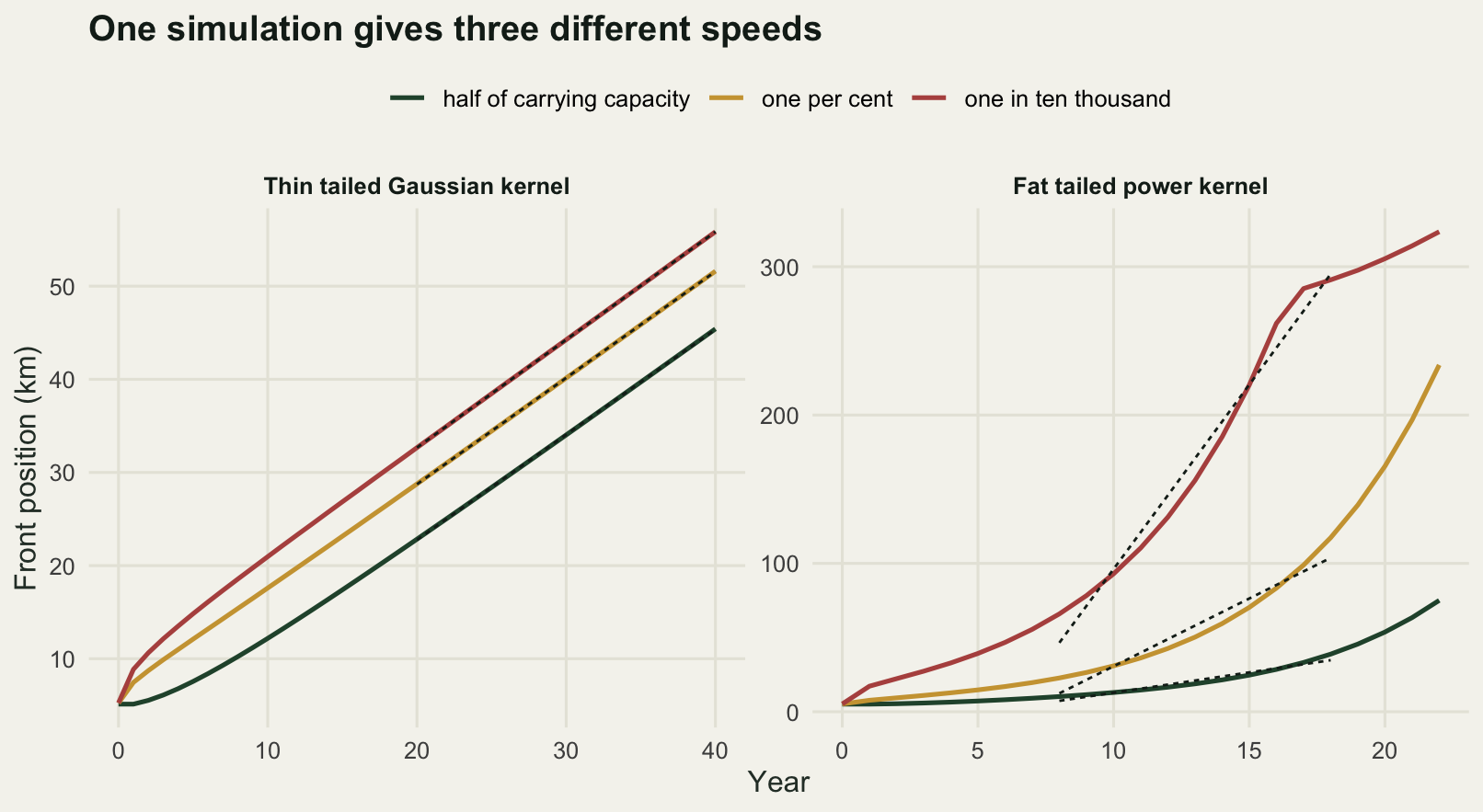
On the thin-tailed run measured late, between years 20 and 40, the three thresholds give 1.1297, 1.1423 and 1.1587 kilometres a year. The standard deviation across the three is 0.0146, or 1.2738 per cent of their mean, and the theory is vindicated: the choice of threshold is worth about one per cent.
Measured early, between years 3 and 13, the same three thresholds give 0.9271, 1.1013 and 1.2288. The standard deviation is 0.1514, which is 13.9481 per cent of the mean, and is 10.3963 times the late figure. The direction of the disagreement matters on its own. The lowest threshold gives 1.2288, which is above the closed form asymptotic speed of 1.1774, so a survey that maps every confirmed record over a decade of a young invasion will report a spread rate faster than the model’s own theoretical maximum. Nothing is wrong with either number. The wave has not finished building its shape, the leading contour is still running ahead of the half density contour, and the difference between contours is still growing.
The fat-tailed panel is where the check stops being a matter of one per cent. Fitted over years 8 to 18, the three thresholds give 2.7403, 9.1329 and 24.8562 kilometres a year. The largest is 9.0707 times the smallest. There is no shared answer to converge to, because an accelerating front has no fixed shape, so the contours separate for ever and each one has its own apparent rate. The straight line fits have an R squared of 0.94624, 0.94363 and 0.97688. A referee looking at the fit statistic alone would accept all three, and would have no way of knowing that the model behind them has no constant speed at all. The thin-tailed fits, for comparison, have an R squared of 0.99998, 0.99999 and 1.00000, so the fit statistic does not separate the two cases either.
The practical form of this check is dull and works: state the threshold, and refit the speed at two or three thresholds. If the answers move by more than a few per cent, you are either in the transient or the front is accelerating, and in both cases a single speed is the wrong summary.
Check 2: the lag phase does not identify itself
Invasion records very often show a lag: years in which the species is known to be present but the mapped extent barely moves, followed by a phase of steady spread. Lags carry a lot of interpretive weight, because a genuine demographic lag means the population is limited at low density, which in turn means that suppressing density is a control option. If the lag is an artefact of not finding the plant, no such conclusion follows.
The check builds a genuine lag and then asks whether a model without one can produce the same map. The genuine version has an Allee effect from mate finding: a fraction of reproduction is independent of density, the rest requires a mate, and mate finding follows a saturating function of local density with a half saturation of 0.2. With a density independent fraction of 0.55 and a multiplication rate of two, the low density growth rate is 1.1 a year, so a small founder population takes many years to build up. Detection is generous throughout: the map records everywhere the density exceeds one fiftieth of carrying capacity.
The rival is the same model with no Allee effect and a founder small enough to be invisible at first. Its multiplication rate and its founding density are both fitted, by least squares, to the mapped extent series produced by the Allee model. The question is how close it can get.
d_map <- 0.02
t_lag <- 40
yrs <- 0:t_lag
g_allee <- grow_allee(r_low, 0.55, 0.2)
obs_ext <- function(sim) {
  f <- fseries(sim, d_map, wd)
  f[is.na(f)] <- 0
  pmax(f, 0)
}
round(c(map_threshold = d_map, allee_half_saturation = 0.2,
        density_independent_share = 0.55, founder_density = 0.005,
        years = t_lag, late_window_start = 25), 4)
map_threshold allee_half_saturation density_independent_share
0.020 0.200 0.550
founder_density years late_window_start
0.005 40.000 25.000 ext_allee <- obs_ext(run_ide(blk(wd, 2, 0.005), k_thin, g_allee, t_lag, wd))
ext_plain <- function(par) obs_ext(run_ide(blk(wd, 2, exp(par[2])), k_thin,
grow_bh(1 + exp(par[1])), t_lag, wd))
fit <- optim(c(log(0.4), log(1e-4)), function(par) sum((ext_plain(par) - ext_allee)^2),
control = list(reltol = 1e-8, maxit = 200))
r_fit <- 1 + exp(fit$par[1])
amp_fit <- exp(fit$par[2])
ext_rival <- ext_plain(fit$par)
sim_est <- run_ide(blk(wd, 90, 1), k_thin, g_allee, 100, wd)
c_allee <- slope_win(fseries(sim_est, 0.5, wd), 60:100)
sl_full <- slope_win(ext_allee, yrs)
sl_late <- slope_win(ext_allee, 25:40)
c(first_detection_allee = min(yrs[ext_allee > 0]),
first_detection_rival = min(yrs[ext_rival > 0]))first_detection_allee first_detection_rival
21 21 round(c(true_growth = r_low, true_low_density_growth = r_low * 0.55,
fitted_growth = r_fit, fitted_founder = amp_fit), 5) true_growth true_low_density_growth fitted_growth
2.00000 1.10000 1.13233
fitted_founder
0.00436 round(c(rmse_km = sqrt(mean((ext_rival - ext_allee)^2)),
max_gap_km = max(abs(ext_rival - ext_allee)),
final_extent_km = ext_allee[t_lag + 1],
max_gap_pct = 100 * max(abs(ext_rival - ext_allee)) / ext_allee[t_lag + 1]), 4) rmse_km max_gap_km final_extent_km max_gap_pct
0.0460 0.1396 13.2400 1.0546 round(c(established_speed = c_allee, slope_with_lag = sl_full,
slope_after_lag = sl_late,
bias_with_lag_pct = 100 * (sl_full / c_allee - 1),
bias_after_lag_pct = 100 * (sl_late / c_allee - 1),
bias_ratio = (1 - sl_full / c_allee) / (1 - sl_late / c_allee)), 4) established_speed slope_with_lag slope_after_lag bias_with_lag_pct
0.5908 0.3564 0.5565 -39.6791
bias_after_lag_pct bias_ratio
-5.8053 6.8349 lag_df <- rbind(
data.frame(year = yrs, extent = ext_allee, model = "Mate finding Allee effect"),
data.frame(year = yrs, extent = ext_rival, model = "Best fitting model with no Allee effect"))
lag_df$model <- factor(lag_df$model,
levels = c("Mate finding Allee effect",
"Best fitting model with no Allee effect"))
fit_full <- lm(ext_allee ~ yrs)
fit_late <- lm(ext_allee[26:41] ~ I(25:40))
line_df <- rbind(
data.frame(year = yrs, extent = as.numeric(fitted(fit_full)),
fitted_on = "Every year, lag included"),
data.frame(year = 25:40, extent = as.numeric(fitted(fit_late)),
fitted_on = "Years 25 to 40 only"))
ggplot(lag_df, aes(year, extent)) +
geom_line(aes(colour = model, linetype = model), linewidth = 0.7) +
geom_line(data = line_df, aes(group = fitted_on, linewidth = fitted_on),
colour = te_pal$ink, linetype = "44") +
scale_colour_manual(values = c(te_pal$forest, te_pal$clay), name = NULL) +
scale_linetype_manual(values = c("solid", "31"), name = NULL) +
scale_linewidth_manual(values = c(0.5, 1.2), name = NULL) +
guides(colour = guide_legend(order = 1, nrow = 2),
linetype = guide_legend(order = 1, nrow = 2),
linewidth = guide_legend(order = 2, nrow = 2)) +
labs(x = "Year", y = "Mapped extent (km)",
title = "A demographic lag and a detection lag draw the same map",
subtitle = paste("The line fitted to years 25 to 40 runs along both extent",
"curves, so it is hard to separate there")) +
theme_te() +
theme(legend.position = "top", legend.box = "horizontal",
plot.subtitle = element_text(size = 9.5, colour = "#2c3a31"))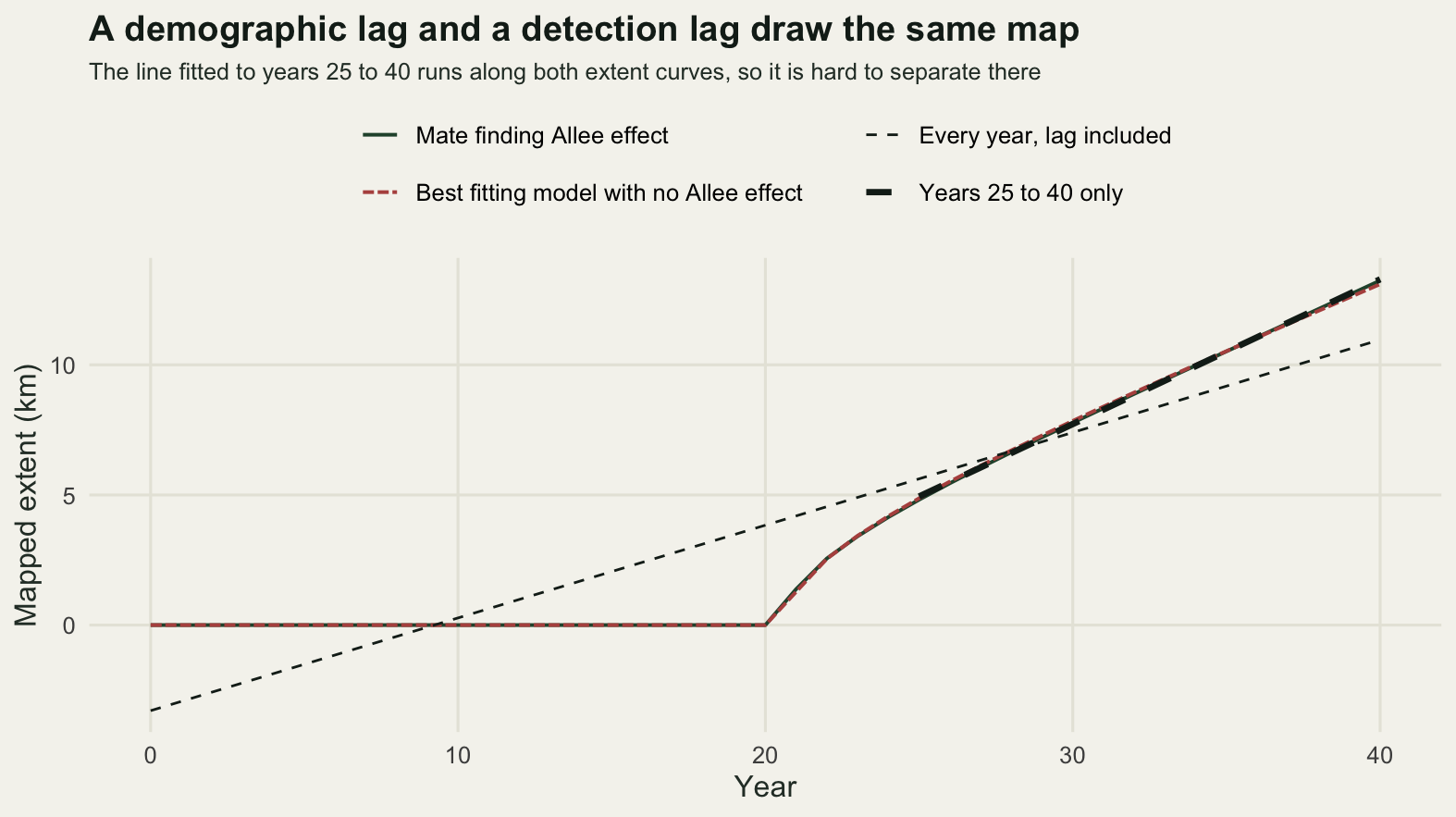
The rival fits. Both series show nothing at all until year 21 and then rise together, and the largest gap between them anywhere in the series is 0.1396 kilometres, on an extent that reaches 13.24 kilometres, so 1.0546 per cent of the final value. The root mean square difference is 0.046 kilometres. No records centre in the world maps an invasion to a tenth of a kilometre. On this evidence the two mechanisms are the same hypothesis.
They are not the same ecology. The truth here multiplies by 2 at low density in the absence of mate limitation and has an Allee effect; the fitted rival multiplies by 1.13233 and has none. What the fit has recovered is the effective low density growth rate of the Allee model, which is 1.1, and that is the only thing the lag phase contains. The Allee effect itself, the property that would tell a manager that pushing density down could stop the invasion outright, leaves no trace in the mapped extent. A model comparison on these data would choose on parsimony, not on evidence.
The second half of the check is cheaper and just as damaging. Fitting a straight line to the whole extent series, lag years included, gives 0.3564 kilometres a year. The established wave in this same model travels at 0.5908. Including the lag in the regression understates the spread rate by 39.6791 per cent. Dropping the lag years and fitting years 25 to 40 gives 0.5565, which is still 5.8053 per cent low because the wave is still building, but the bias has shrunk by a factor of 6.8349. A speed fitted through a lag phase is not an estimate of anything: it is an average of two regimes, weighted by how long the survey happened to run before the invasion took off.
Check 3: the detection delay
Now the opposite problem. The population is well established, spreading steadily, and the surveyor is imperfect. Survey points sit every two kilometres along the corridor, and at each one the probability of detection rises with local density as one minus the exponential of minus twenty times that density, so a point at one twentieth of carrying capacity is found with probability 0.6321 and a point at one five-hundredth with probability 0.0392. The observed front is the furthest survey point with a detection, over 400 independent survey years.
The true front is taken at a density of one thousandth, which is where the plant is genuinely present and essentially never found. The question is not whether the observed front lags, because it must. The question is whether the lag is constant, because a constant lag biases the position and leaves the slope alone, and a lag that grows biases both.
set.seed(20260728)
n_rep <- 400
lam_det <- 20
cell_x <- seq(-20, 400, by = 2)
cell_i <- round((cell_x - wd$x[1]) / wd$h) + 1
d_true <- 1e-3

n_show <- 30
c(survey_replicates = n_rep, survey_spacing_km = 2, detection_lambda = lam_det,
  replicates_drawn = n_show)
survey_replicates survey_spacing_km detection_lambda replicates_drawn
400 2 20 30 print(c(true_front_density = d_true))true_front_density
0.001 obs_fronts <- function(sim, times) {
pd <- 1 - exp(-lam_det * sim[times + 1, cell_i, drop = FALSE])
t(sapply(seq_along(times), function(k) {
hit <- matrix(runif(n_rep * length(cell_x)), n_rep) < rep(pd[k, ], each = n_rep)
apply(hit, 1, function(h) if (any(h)) max(cell_x[h]) else NA_real_)
}))
}
det_summary <- function(sim, tmax, win) {
times <- 0:tmax
of <- obs_fronts(sim, times)
mo <- rowMeans(of)
tf <- fseries(sim, d_true, wd)
band <- t(apply(of, 1, quantile, c(0.1, 0.9)))
list(times = times, obs = mo, true = tf, lag = tf - mo, mat = of,
spread = mean(apply(of, 1, sd_few)[win + 1]),
band = mean((band[, 2] - band[, 1])[win + 1]),
ahead = mean((rowMeans(of > tf))[win + 1]),
s_true = slope_win(tf, win), s_obs = slope_win(mo, win),
lag_mean = mean((tf - mo)[win + 1]), lag_trend = slope_win(tf - mo, win))
}
det_thin <- det_summary(sim_thin, 40, 20:40)
det_fat <- det_summary(sim_fat, 22, 8:18)
round(c(detected_at_5_pct_density = 1 - exp(-lam_det * 0.05),
detected_at_0_2_pct_density = 1 - exp(-lam_det * 0.002)), 4) detected_at_5_pct_density detected_at_0_2_pct_density
0.6321 0.0392 print(round(rbind(year = det_thin$times, true = det_thin$true,
observed = det_thin$obs, lag = det_thin$lag)[, seq(1, 41, by = 8)], 3)) [,1] [,2] [,3] [,4] [,5] [,6]
year 0.00 8.000 16.000 24.000 32.000 40.000
true 5.25 17.106 26.263 35.425 44.619 53.841
observed 4.00 13.480 22.190 31.185 40.385 49.530
lag 1.25 3.626 4.073 4.240 4.234 4.311print(round(rbind(year = det_fat$times, true = det_fat$true,
observed = det_fat$obs, lag = det_fat$lag)[, c(1, 4, 7, 10, 13, 16, 19, 23)], 3)) [,1] [,2] [,3] [,4] [,5] [,6] [,7] [,8]
year 0.00 3.000 6.000 9.000 12.000 15.000 18.000 22.000
true 5.25 16.565 27.314 44.796 74.313 124.210 208.360 295.618
observed 4.00 10.090 17.785 30.150 61.430 112.695 195.095 275.605
lag 1.25 6.475 9.529 14.646 12.883 11.515 13.265 20.013round(c(thin_true_speed = det_thin$s_true, thin_observed_speed = det_thin$s_obs,
thin_speed_bias_pct = 100 * (det_thin$s_obs / det_thin$s_true - 1),
thin_mean_lag_km = det_thin$lag_mean, thin_lag_trend = det_thin$lag_trend,
thin_lag_years = det_thin$lag_mean / det_thin$s_true,
thin_trend_over_speed = det_thin$lag_trend / det_thin$s_true,
thin_replicate_sd_km = det_thin$spread,
thin_band_10_90_km = det_thin$band,
thin_share_ahead = det_thin$ahead), 4) thin_true_speed thin_observed_speed thin_speed_bias_pct
1.1500 1.1423 -0.6651
thin_mean_lag_km thin_lag_trend thin_lag_years
4.2115 0.0076 3.6623
thin_trend_over_speed thin_replicate_sd_km thin_band_10_90_km
0.0067 1.4797 3.3333
thin_share_ahead
0.0090 round(c(fat_true_speed = det_fat$s_true, fat_observed_speed = det_fat$s_obs,
fat_speed_bias_pct = 100 * (det_fat$s_obs / det_fat$s_true - 1),
fat_lag_min_km = min(det_fat$lag), fat_lag_max_km = max(det_fat$lag),
fat_lag_trend = det_fat$lag_trend,
fat_lag_share_early_pct = 100 * det_fat$lag[7] / det_fat$true[7],
fat_lag_share_late_pct = 100 * det_fat$lag[19] / det_fat$true[19],
fat_band_10_90_km = det_fat$band,
fat_share_ahead = det_fat$ahead), 4) fat_true_speed fat_observed_speed fat_speed_bias_pct
16.4657 16.8630 2.4126
fat_lag_min_km fat_lag_max_km fat_lag_trend
1.2497 40.8081 -0.3973
fat_lag_share_early_pct fat_lag_share_late_pct fat_band_10_90_km
34.8879 6.3663 77.7091
fat_share_ahead
0.2543 det_df <- rbind(
data.frame(year = det_thin$times, lag = det_thin$lag,
kernel = "Thin tailed Gaussian kernel"),
data.frame(year = det_fat$times, lag = det_fat$lag,
kernel = "Fat tailed power kernel"))
rep_df <- rbind(
data.frame(year = rep(det_thin$times, n_show),
lag = as.vector(det_thin$true - det_thin$mat[, seq_len(n_show)]),
rep_id = rep(seq_len(n_show), each = length(det_thin$times)),
kernel = "Thin tailed Gaussian kernel"),
data.frame(year = rep(det_fat$times, n_show),
lag = as.vector(det_fat$true - det_fat$mat[, seq_len(n_show)]),
rep_id = rep(seq_len(n_show), each = length(det_fat$times)),
kernel = "Fat tailed power kernel"))
lv <- c("Thin tailed Gaussian kernel", "Fat tailed power kernel")
det_df$kernel <- factor(det_df$kernel, levels = lv)
rep_df$kernel <- factor(rep_df$kernel, levels = lv)
ggplot(det_df, aes(year, lag)) +
geom_line(data = rep_df, aes(group = rep_id), colour = te_pal$sage,
alpha = 0.5, linewidth = 0.3) +
geom_hline(yintercept = 0, colour = te_pal$ink, linetype = "22", linewidth = 0.5) +
geom_line(colour = te_pal$forest, linewidth = 1.1) +
facet_wrap(~kernel, scales = "free") +
labs(x = "Year", y = "True front minus observed front (km)",
title = "The lag settles only when the front has a settled shape") +
theme_te() +
theme(strip.text = element_text(colour = te_pal$ink, face = "bold"))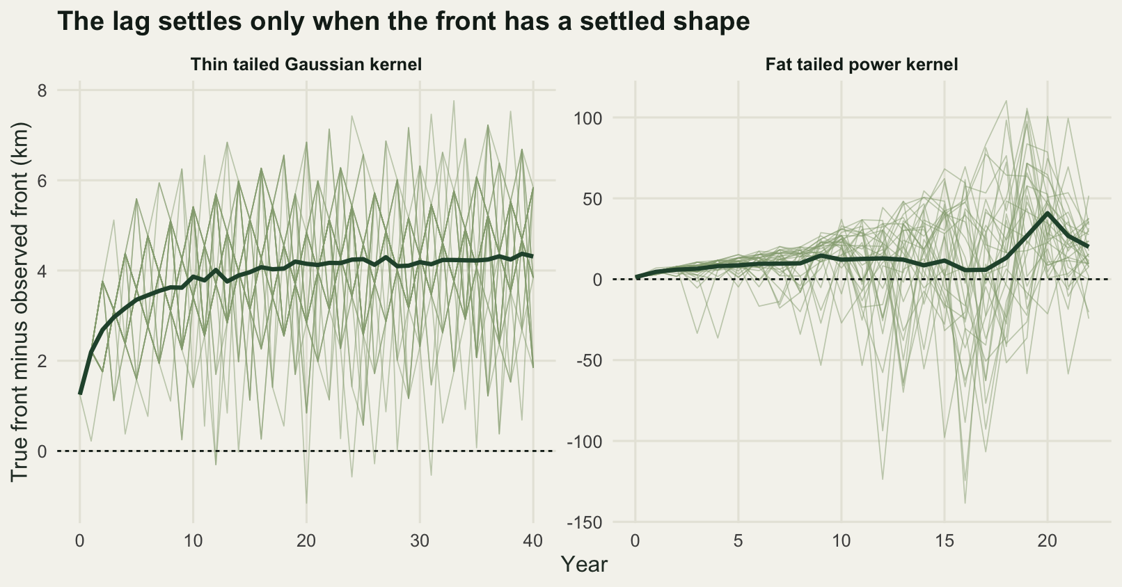
On the thin-tailed run the answer is the reassuring one. The true front advances at 1.15 kilometres a year and the observed front at 1.1423, a bias of 0.6651 per cent, which is inside the replicate noise. The lag settles at 4.2115 kilometres and stays there: regressed on year over the measurement window its trend is 0.0076 kilometres a year, which is 0.0067 of the speed itself. A travelling wave has a fixed shape, the detection probability depends only on density, so the distance from the leading contour to the last point the surveyor finds is a property of the shape and not of time. The rate is recoverable and the position is not.
That is not a small caveat. The 4.2115 kilometre offset converts into time at the front’s own speed: the plant reaches any given bridge or reserve boundary 3.6623 years before the map shows it there. A quarantine line drawn on the observed front is already behind the invasion when it is drawn, by an amount the fitted speed gives no hint of, and the standard deviation of the observed front across survey replicates is 1.4797 kilometres, so a single year’s map cannot even measure the offset. The band between the tenth and ninetieth percentiles of survey outcomes is 3.3333 kilometres wide, and the survey puts the front ahead of its true position in 0.009 of survey years, so the direction of the error at least is dependable.
The fat-tailed run behaves differently, and not in the direction I expected. The lag never settles. It runs from 1.2497 kilometres in the first year to 14.646 by year 9, falls back to 11.515 by year 15, and then spikes to a maximum of 40.8081 before dropping back to 20.013 by year 22, because the front is accelerating away from its own tail and the shape ahead of the leading contour keeps changing. Fitted over years 8 to 18 the lag even trends downwards in this simulation, at minus 0.3973 kilometres a year, which is an artefact of that dip. Relative to the front position the lag shrinks through the middle of the run: 34.8879 per cent of the true position at year 6, 6.3663 per cent at year 18. It does not shrink at either end: the share rises over the first few years, and the late spike lifts it again after year 18. On this run the slope of the observed front over years 8 to 18 comes out 2.4126 per cent above the true slope, not below it.
The replicates are the sharper part of the picture. The band between the tenth and ninetieth percentiles of survey outcomes is 77.7091 kilometres wide, against 3.3333 kilometres in the thin-tailed run, and in 0.2543 of survey years the observed front is not behind the true front at all but ahead of it, because a single detected outlier in the tail throws the mapped boundary far forward. The lesson is not that the bias has a known sign. With an accelerating front the lag is a moving target, one year’s map is nearly uninformative about the front’s position, and no single correction fixes either problem.
Check 4: an Allee effect stops the wave and the formula does not notice
Everything so far has assumed the linear theory. The closed form speed comes from linearising the model at zero density, on the argument that the front is pulled by the individuals furthest ahead, who are at densities so low that nothing density dependent matters to them. An Allee effect breaks that argument at its root, because at low density the per capita growth rate is not at its maximum but at its minimum.
The sweep uses the mate finding model again, with the density independent share of reproduction running from 1, meaning no Allee effect at all, down to 0.13, meaning almost all reproduction needs a mate. The linearised prediction uses the low density multiplication rate, which is the density independent share times two, and exists only while that product exceeds one. Each point is a run of 100 years started from a wide block at the upper equilibrium, with the speed measured between years 60 and 100 at half the local equilibrium density.
eq_hi <- function(ss) {
  f <- grow_allee(r_low, ss, 0.2)
  op <- optimize(function(n) f(n) - n, c(0.01, 5), maximum = TRUE)
  if (op$objective <= 0) return(NA_real_)
  uniroot(function(n) f(n) - n, c(op$maximum, 5), tol = 1e-10)$root
}
eq_lo <- function(ss) {
  if (r_low * ss >= 1) return(NA_real_)
  f <- grow_allee(r_low, ss, 0.2)
  op <- optimize(function(n) f(n) - n, c(0.01, 5), maximum = TRUE)
  uniroot(function(n) f(n) - n, c(1e-10, op$maximum), tol = 1e-12)$root
}
speed_allee <- function(ss) {
  ns <- eq_hi(ss)
  sim <- run_ide(blk(wd, 90, ns), k_thin, grow_allee(r_low, ss, 0.2), 100, wd)
  slope_win(fseries(sim, ns / 2, wd), 60:100)
}
c_lin <- function(ss) if (r_low * ss > 1) sqrt(2 * sd_kern^2 * log(r_low * ss)) else NA_real_

c(years_per_run = 100, window_start = 60, window_end = 100)
years_per_run window_start window_end
100 60 100 sh <- c(seq(0.13, 0.3, by = 0.01), seq(0.35, 0.5, by = 0.05),
seq(0.51, 0.54, by = 0.01), seq(0.55, 1, by = 0.05))
sweep <- data.frame(share = sh, upper = sapply(sh, eq_hi), lower = sapply(sh, eq_lo),
measured = sapply(sh, speed_allee), linear = sapply(sh, c_lin))
sweep$ratio <- sweep$measured / sweep$linear
keep <- round(sweep$share, 2) %in% c(0.13, 0.15, 0.17, 0.2, 0.3, 0.5, 0.55, 0.6, 0.65,
0.7, 0.8, 1)
print(round(sweep[keep, ], 4), row.names = FALSE) share upper lower measured linear ratio
0.13 0.5095 0.2905 -0.0996 NA NA
0.15 0.5414 0.2586 -0.0442 NA NA
0.17 0.5673 0.2327 0.0022 NA NA
0.20 0.6000 0.2000 0.0631 NA NA
0.30 0.6828 0.1172 0.2308 NA NA
0.50 0.8000 NA 0.5192 NA NA
0.55 0.8243 NA 0.5908 0.4366 1.3531
0.60 0.8472 NA 0.6640 0.6039 1.0996
0.65 0.8690 NA 0.7391 0.7244 1.0204
0.70 0.8899 NA 0.8144 0.8203 0.9928
0.80 0.9292 NA 0.9527 0.9695 0.9826
1.00 1.0000 NA 1.1592 1.1774 0.9845s_stop <- uniroot(speed_allee, c(0.15, 0.19), tol = 1e-5)$root
round(c(share_where_wave_stops = s_stop,
allee_threshold_there = eq_lo(s_stop) / eq_hi(s_stop),
linear_theory_says_stops_at = 1 / r_low,
measured_speed_when_linear_says_zero = speed_allee(0.5),
share_of_unimpaired_speed_pct = 100 * speed_allee(0.5) / sweep$measured[nrow(sweep)],
stop_criterion_ratio = 0.5 / s_stop,
retreat_speed_at_0_13 = sweep$measured[1]), 5) share_where_wave_stops allee_threshold_there
0.16897 0.41319
linear_theory_says_stops_at measured_speed_when_linear_says_zero
0.50000 0.51918
share_of_unimpaired_speed_pct stop_criterion_ratio
44.78948 2.95915
retreat_speed_at_0_13
-0.09960 lin_x <- seq(0.5, 1, length.out = 501)
lin_y <- vapply(lin_x, c_lin, numeric(1))
lin_y[is.na(lin_y)] <- 0
allee_df <- rbind(
data.frame(share = sweep$share, speed = sweep$measured, kind = "Measured in the simulation"),
data.frame(share = lin_x, speed = lin_y, kind = "Linearised prediction"))
allee_df <- allee_df[!is.na(allee_df$speed), ]
ggplot(allee_df, aes(share, speed, colour = kind, linetype = kind)) +
geom_hline(yintercept = 0, colour = te_pal$line, linewidth = 0.8) +
geom_vline(xintercept = s_stop, colour = te_pal$ink, linetype = "22", linewidth = 0.5) +
geom_line(linewidth = 1) +
annotate("text", x = s_stop + 0.02, y = 0.95, hjust = 0, size = 3.4, colour = te_pal$ink,
label = "wave stops here") +
annotate("text", x = 0.545, y = 0.13, hjust = 0, size = 3.4, colour = te_pal$clay,
label = "linearised speed reaches zero,\nand the formula ends here") +
scale_colour_manual(values = c(te_pal$clay, te_pal$forest), name = NULL) +
scale_linetype_manual(values = c("31", "solid"), name = NULL) +
labs(x = "Density independent share of reproduction",
y = "Front speed (km per year)",
title = "The linearised formula stops the wave far too early") +
theme_te() +
theme(legend.position = "top")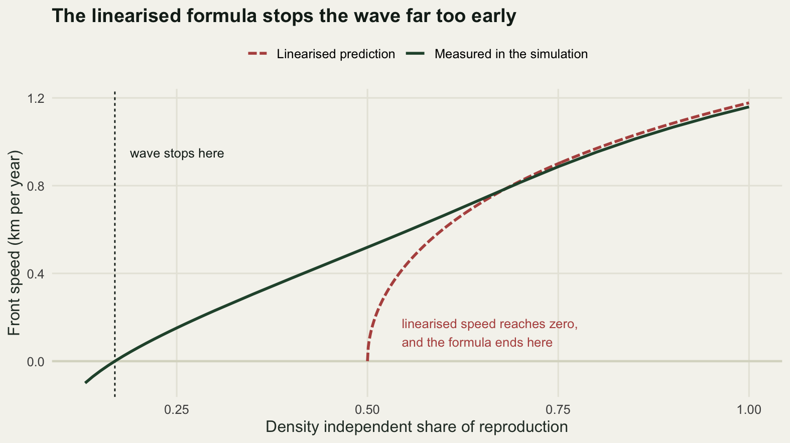
Three results sit in that table. On the right hand side, where the Allee effect is mild, the measured speed tracks the linearised prediction: the ratio is 0.9845 with no Allee effect at all and 0.9826 at a share of 0.8, and that shortfall is the same logarithmic transient measured in the opening section, not a failure of the formula. Somewhere between shares of 0.7 and 0.65 the ratio crosses one, reaching 1.0204 at 0.65 and 1.3531 at 0.55. The front has stopped being pulled by its leading edge and is being pushed by the bulk behind it, which travels faster than the tail can on its own. Past that point the linearised formula is not conservative in either direction; it is simply not describing the same object.
The second result is the one that matters for management. The linearised theory says the wave stops when the low density growth rate falls to one, which here is a density independent share of 0.5. At that share the simulated wave is still advancing at 0.51918 kilometres a year, which is 44.78948 per cent of the speed with no Allee effect at all. The wave does not actually stop until the share falls to 0.16897, and below that it reverses: at a share of 0.13 the front retreats at 0.09960 kilometres a year, so the occupied stretch of river shrinks year on year with no management at all. The mate finding failure needed to halt the invasion is 2.95915 times as severe as the linearised criterion suggests.
The third result is a rule of thumb worth keeping. At the share where the wave stops, the unstable lower equilibrium sits at 0.41319 of the upper one. That is the discrete time analogue of the classical result for reaction diffusion, where the wave reverses when the Allee threshold passes half of carrying capacity. It is a far more useful diagnostic than the linearised speed, because it depends only on the growth function and can be read off without simulating anything: compare the Allee threshold with the carrying capacity, and if the ratio is anywhere near a half, the linearised speed formula is not applicable to the population you have.
The honest limit
The largest weakness is the one measured in the opening section, and it is not a bug. In the fat-tailed runs, the front position after 22 years moves by a factor of 7.7495 as the density floor moves from one part in a million to one part in a trillion. A deterministic integrodifference model has no individuals in it, so it has no natural place to stop counting, and for an accelerating front the answer depends on where you do stop. Checks 1 and 3 both use those runs, so their fat-tailed numbers are conditional on a floor of one part in a billion. The thin-tailed numbers are not: the largest shift they show across the same six orders of magnitude is 0.3988 kilometres, on fronts that have travelled tens of kilometres. Any serious use of an accelerating spread model has to make the floor explicit and defend it as a density of one individual, which means it has to be tied to real areas and real population sizes rather than chosen for numerical comfort.
Two further limits are structural. The model is deterministic, so the spread of the observed front across replicates in check 3 comes only from the survey, not from the population; a stochastic front wanders as well, and the wander is often larger than anything measured here. And the model is one dimensional, which is defensible for a river corridor or a road verge and wrong for a spreading patch in a landscape, where the front is a curve and its curvature slows it.
The deeper limit applies to all four checks equally. Each of them tests a decision made inside an agreed model: where the front is, which years to fit, how detection works, whether the growth function has an Allee term. None of them tests whether spread happens by local diffusion at all. A population that mostly moves by hitchhiking on vehicles passes every check in this post, since it will produce a front, a lag, a detection delay and a response to an Allee term, and every diagnostic here will return an interpretable number for a process that is not happening.
Where to go next
The first thing to do with an existing spread estimate is the cheapest check here: refit the speed at two more density thresholds, and refit it dropping the first third of the series. If either changes the answer by more than a few per cent, the single speed should not leave the office.
For the mechanism that check 4 turns on, Allee effects and thresholds sets out the growth functions and the critical densities in a non-spatial setting, and checking an Allee analysis shows how hard the threshold is to estimate from field data, which is the estimate this post has just made load-bearing. For the case where the front is not a front at all, long-distance jumps and stratified spread treats the population as a main wave plus a scatter of new colonies, where the mapped boundary means something different again.
References
Kot M, Lewis MA, van den Driessche P 1996 Ecology 77(7):2027-2042 (10.2307/2265698)
Lewis MA, Kareiva P 1993 Theoretical Population Biology 43(2):141-158 (10.1006/tpbi.1993.1007)
Wang MH, Kot M, Neubert MG 2002 Journal of Mathematical Biology 44(2):150-168 (10.1007/s002850100116)
Melbourne BA, Hastings A 2009 Science 325(5947):1536-1539 (10.1126/science.1176138)
Brunet E, Derrida B 1997 Physical Review E 56(3):2597-2604 (10.1103/PhysRevE.56.2597)
Kot M 2001 Elements of Mathematical Ecology. Cambridge University Press, ISBN 978-0-521-00150-2