library(ggplot2)
library(patchwork)

te_paper  <- "#f5f4ee"
te_ink    <- "#16241d"
te_body   <- "#2c3a31"
te_forest <- "#275139"
te_rust   <- "#b5534e"
te_gold   <- "#c9b458"
te_line   <- "#dad9ca"

theme_datasheet <- function() {
  theme_minimal(base_size = 12) +
    theme(plot.background  = element_rect(fill = te_paper, colour = NA),
          panel.background = element_rect(fill = te_paper, colour = NA),
          panel.grid.major = element_line(colour = te_line, linewidth = 0.3),
          panel.grid.minor = element_blank(),
          text             = element_text(colour = te_body),
          plot.title       = element_text(colour = te_ink, face = "bold"),
          plot.subtitle    = element_text(colour = te_body),
          axis.text        = element_text(colour = te_body))
}Critical patch size and the dispersal kernel
R
dispersal
population dynamics
spatial ecology
simulation
ecology tutorial
Critical patch size in R: eigenvalues show a peaked dispersal kernel needs less habitat than a Gaussian, and demographic noise lifts the practical threshold.
A flightless ground beetle lives on the grassy margin between a river and an arable field. The margin is a strip a few metres wide and a few hundred metres long, and a restoration scheme is about to cut it into reaches, some kept as grassland and some ploughed. Larvae that end up on bare soil die. A planner asks the question that every strip habitat eventually raises: how long does a reach have to be before the beetle can hold it on its own?
The textbook answer is old. Skellam (1951) showed that a population which grows inside a patch and diffuses out of it into lethal surroundings has a critical patch size. Below it, losses over the edge outrun local growth and the population dies however large it starts; above it, the population persists. For diffusion the threshold has a closed form that needs only the growth rate and the diffusion coefficient. What it does not need, and cannot see, is the shape of the dispersal kernel.
This site already has a small cluster on integrodifference models, and all of it points outwards. The speed of an invasion front steps a Gaussian kernel forward along a corridor and checks the front speed against the closed form from the moment generating function. Fat tails and accelerating spread shows that a front driven by a kernel with no moment generating function never settles at a constant speed, and checking an invasion spread model tests the density threshold, the lag phase and the Allee effect on the same kind of model. Every one of those posts asks how fast a population moves into open space. This one uses the same redistribution operator on a bounded patch, where leaving is death, and asks how much space a population needs.
The post measures three things. It computes the critical length for a Gaussian and a Laplace kernel with the same variance, by finding the dominant eigenvalue of the discretised operator, and checks the integrator against the two closed forms that exist. It sets the patch-size ranking of the two kernels beside their front-speed ranking over a range of growth rates. Then it runs an individual-based version with Poisson offspring and asks how far above the deterministic threshold a patch has to be before a finite population actually persists.
Two kernels with the same variance
All lengths below are in units of the dispersal standard deviation, so a patch of length three is three standard deviations of one generation’s displacement. The two kernels are a Gaussian and a Laplace (double exponential) distribution. The Laplace density is \(\tfrac{\alpha}{2} e^{-\alpha |x|}\), and its variance is \(2/\alpha^2\), so matching a standard deviation of one needs \(\alpha = \sqrt{2}\). The Laplace kernel is not fat tailed in the sense of the accelerating spread post: its tail is exponential and its moment generating function exists. What differs is the shape near zero. It is sharply peaked, so it keeps more offspring close to the parent and pays for the same variance with more moderately long moves.
sd_disp <- 1                          # dispersal standard deviation (length unit)
alpha_lap <- sqrt(2) / sd_disp        # Laplace rate giving the same variance
r0_main <- 1.5                        # offspring per adult at low density

cdf_kern <- list(
  Gaussian = function(d) pnorm(d, 0, sd_disp),
  Laplace  = function(d) ifelse(d < 0, 0.5 * exp(alpha_lap * d),
                                1 - 0.5 * exp(-alpha_lap * d)))

set.seed(3017)
n_draw <- 200000
draw_lap <- rexp(n_draw, alpha_lap) * (2 * (runif(n_draw) < 0.5) - 1)
sd_lap_draw <- sd(draw_lap)
med_gau <- qnorm(0.75, 0, sd_disp)
med_lap <- log(2) / alpha_lap
The matching is worth one check before anything depends on it. 200000 Laplace draws with \(\alpha = \sqrt{2}\) have a standard deviation of 1.0041. The two kernels part company in the median distance moved: 0.674 standard deviations for the Gaussian and 0.490 for the Laplace.
The population model is the linear integrodifference equation on a patch \([0, L]\) with lethal surroundings, \(n_{t+1}(x) = R_0 \int_0^L k(x - y)\, n_t(y)\, \mathrm{d}y\), which is what any model with density dependence reduces to at low density. The population grows when the dominant eigenvalue of the operator exceeds one. Discretising the patch into cells turns the operator into a matrix, and the critical length \(L^*\) is where \(R_0\) times the largest eigenvalue of that matrix equals one. Each matrix entry integrates the kernel exactly over the source cell with the distribution function, which matters for the Laplace kernel: its cusp at zero would be sampled badly by evaluating the density at cell midpoints.
lambda_max <- function(patch_len, kern, n_cell) {
  h_cell <- patch_len / n_cell
  x_mid  <- (seq_len(n_cell) - 0.5) * h_cell
  gap    <- outer(x_mid, x_mid, "-")
  op_mat <- cdf_kern[[kern]](gap + h_cell / 2) - cdf_kern[[kern]](gap - h_cell / 2)
  eigen(op_mat, symmetric = TRUE, only.values = TRUE)$values[1]
}

critical_len <- function(kern, r0, n_cell) {
  uniroot(function(len) r0 * lambda_max(len, kern, n_cell) - 1,
          c(0.02, 40), tol = 1e-8)$root
}

lap_closed  <- 2 / (alpha_lap * sqrt(r0_main - 1)) * atan(1 / sqrt(r0_main - 1))
kiss_closed <- pi * sqrt((sd_disp^2 / 2) / log(r0_main))

n_check <- c(50, 100, 200)
conv_tab <- data.frame(
  n_cell   = n_check,
  laplace  = vapply(n_check, function(m) critical_len("Laplace", r0_main, m), 0),
  gaussian = vapply(n_check, function(m) critical_len("Gaussian", r0_main, m), 0))
conv_tab$lap_error <- conv_tab$laplace - lap_closed

kiss_linear <- pi * sqrt((sd_disp^2 / 2) / (r0_main - 1))   # diffusion threshold with r = R0 - 1

n_main    <- 200
lstar_gau <- conv_tab$gaussian[conv_tab$n_cell == n_main]
lstar_lap <- conv_tab$laplace[conv_tab$n_cell == n_main]
gau_drift <- abs(diff(conv_tab$gaussian[conv_tab$n_cell >= 100]))
ratio_lap_gau  <- lstar_lap / lstar_gau
ratio_gau_kiss <- lstar_gau / kiss_closed
ratio_gau_kiss_lin <- lstar_gau / kiss_linear
Two closed forms are available to test the integrator. For the Laplace kernel Kot and Schaffer (1986) showed that the integral equation is equivalent to a second order differential equation, whose solutions are cosines; the eigenvalue belonging to a cosine of frequency \(w\) is \(\alpha^2/(\alpha^2 + w^2)\), and the boundary condition of the integral equation fixes \(\tan(wL/2) = \alpha / w\). Setting \(R_0\alpha^2/(\alpha^2 + w^2) = 1\) gives \(L^* = \frac{2}{\alpha\sqrt{R_0 - 1}} \arctan\!\big(1/\sqrt{R_0 - 1}\big)\). For diffusion with the same variance per generation, \(D = \sigma^2/2\), and growth rate \(r = \log R_0\), Skellam’s diffusion threshold is \(L = \pi\sqrt{D/r}\).
At \(R_0 = 1.5\) the Laplace closed form is 1.910633. The numerical root is off by -8.39e-05 with 50 cells, -2.09e-05 with 100 and -5.24e-06 with 200: the error falls by a factor of four each time the cell width halves, as a second order scheme should. The Gaussian root, which has no closed form, moves by 1.47e-05 between 100 and 200 cells. Everything below uses 200 cells.
The critical lengths are 2.301 standard deviations for the Gaussian kernel and 1.911 for the Laplace, against 3.489 for diffusion. The peaked kernel needs a patch 0.83 times as long as the Gaussian one, and the Gaussian integrodifference threshold is itself 0.66 of the diffusion value, although a Gaussian kernel is exactly what diffusion produces over one generation. The difference lies in what counts as a loss. In the diffusion model an individual dies the moment its path touches the edge, and it grows while it moves. In the integrodifference model only the landing point counts, so an offspring whose path strays outside and comes back is kept.
len_grid <- seq(1, 6, by = 0.25)
eig_df <- rbind(
  data.frame(len = len_grid, kern = "Gaussian",
             growth = r0_main * vapply(len_grid, lambda_max, 0, kern = "Gaussian", n_cell = 120)),
  data.frame(len = len_grid, kern = "Laplace",
             growth = r0_main * vapply(len_grid, lambda_max, 0, kern = "Laplace", n_cell = 120)))
star_df <- data.frame(len = c(lstar_gau, lstar_lap), growth = 1,
                      kern = c("Gaussian", "Laplace"))

ggplot(eig_df, aes(len, growth, colour = kern)) +
  geom_hline(yintercept = 1, colour = te_body, linewidth = 0.5) +
  geom_vline(xintercept = kiss_closed, linetype = "dashed", colour = te_rust, linewidth = 0.7) +
  annotate("text", x = kiss_closed + 0.08, y = 0.55, label = "diffusion threshold",
           hjust = 0, colour = te_rust, size = 3.6) +
  geom_line(linewidth = 1) +
  geom_point(data = star_df, size = 3) +
  scale_colour_manual(values = c(Gaussian = te_forest, Laplace = te_gold), name = NULL) +
  scale_y_continuous(limits = c(0.5, 1.5)) +
  labs(x = "patch length (dispersal standard deviations)",
       y = "growth factor at low density",
       title = "The peaked kernel crosses one sooner",
       subtitle = "points: critical lengths; horizontal line: replacement") +
  theme_datasheet() +
  theme(legend.position = "bottom")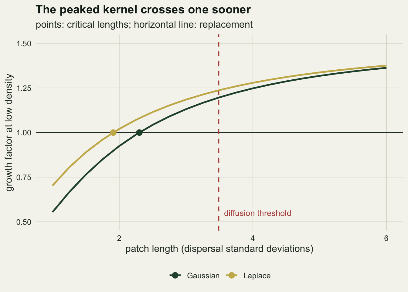
Where the offspring are lost
The reason is visible without any eigenvalues. An offspring born to a parent standing a distance \(d\) from the edge is lost with probability equal to the kernel’s tail beyond \(d\). Both kernels lose exactly half at \(d = 0\), and both lose almost nothing deep inside a long patch. In between they differ, and the difference changes sign.
dist_grid <- seq(0, 3, by = 0.01)
loss_gau <- 1 - cdf_kern$Gaussian(dist_grid)
loss_lap <- 1 - cdf_kern$Laplace(dist_grid)
cross_d  <- uniroot(function(d) (1 - cdf_kern$Gaussian(d)) - (1 - cdf_kern$Laplace(d)),
                    c(0.5, 3))$root
d_show   <- 0.5
loss_gau_half <- 1 - cdf_kern$Gaussian(d_show)
loss_lap_half <- 1 - cdf_kern$Laplace(d_show)

# loss for the whole population at the Gaussian critical length, uniform adults
mean_loss <- function(kern, len) {
  x_par <- seq(0, len, length.out = 2001)
  mean(1 - (cdf_kern[[kern]](len - x_par) - cdf_kern[[kern]](-x_par)))
}
loss_unif_gau <- mean_loss("Gaussian", lstar_gau)
loss_unif_lap <- mean_loss("Laplace", lstar_gau)
A parent 0.5 standard deviations from the edge loses 0.309 of its offspring under the Gaussian kernel and 0.247 under the Laplace. The curves cross at 1.68 standard deviations; beyond that the Laplace kernel loses more, because its variance sits in the longer moves. On a patch of the Gaussian critical length no adult is more than 1.15 standard deviations from an edge, short of the crossing, so the part of the curve where the peaked kernel is kinder is the part that matters. Spread adults evenly over a patch of the Gaussian critical length and the fraction of offspring landing outside is 0.344 under the Gaussian kernel and 0.296 under the Laplace.
loss_df <- rbind(data.frame(dist = dist_grid, loss = loss_gau, kern = "Gaussian"),
                 data.frame(dist = dist_grid, loss = loss_lap, kern = "Laplace"))
ggplot(loss_df, aes(dist, loss, colour = kern)) +
  geom_vline(xintercept = cross_d, linetype = "dashed", colour = te_body, linewidth = 0.5) +
  geom_line(linewidth = 1) +
  scale_colour_manual(values = c(Gaussian = te_forest, Laplace = te_gold), name = NULL) +
  labs(x = "parent's distance from the edge (dispersal standard deviations)",
       y = "share of offspring lost",
       title = "Near the edge the peaked kernel loses less",
       subtitle = "dashed line: where the two loss curves cross") +
  theme_datasheet() +
  theme(legend.position = "bottom")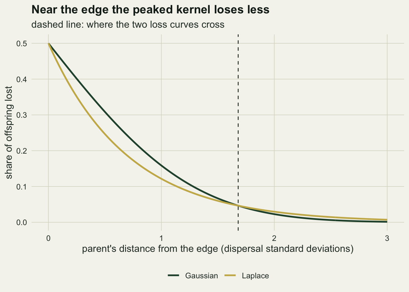
Faster fronts, smaller patches
A reader arriving from the invasion posts might carry over a simple rule: the kernel that spreads faster also bleeds faster from a small patch. The front speed for a kernel with a moment generating function \(M(s)\) is \(c^* = \min_s \log(R_0 M(s))/s\), the formula of Weinberger (1982) checked in the speed post. For the Laplace kernel \(M(s) = \alpha^2/(\alpha^2 - s^2)\) for \(s < \alpha\). Both quantities can be computed over the same range of growth rates.
mgf_log <- list(Gaussian = function(s) s^2 * sd_disp^2 / 2,
                Laplace  = function(s) log(alpha_lap^2 / (alpha_lap^2 - s^2)))
front_speed <- function(kern, r0) {
  s_top <- if (kern == "Gaussian") 30 else alpha_lap - 1e-9
  optimize(function(s) (log(r0) + mgf_log[[kern]](s)) / s, c(1e-6, s_top))$objective
}

r0_grid <- c(1.1, 1.25, 1.5, 2, 3, 5, 10)
rank_tab <- data.frame(r0 = r0_grid)
rank_tab$lstar_gau <- vapply(r0_grid, function(r) critical_len("Gaussian", r, 150), 0)
rank_tab$lstar_lap <- vapply(r0_grid, function(r) critical_len("Laplace", r, 150), 0)
rank_tab$lap_cf    <- 2 / (alpha_lap * sqrt(r0_grid - 1)) * atan(1 / sqrt(r0_grid - 1))
rank_tab$kiss      <- pi * sqrt((sd_disp^2 / 2) / log(r0_grid))
rank_tab$c_gau     <- vapply(r0_grid, function(r) front_speed("Gaussian", r), 0)
rank_tab$c_lap     <- vapply(r0_grid, function(r) front_speed("Laplace", r), 0)
rank_tab$len_ratio <- rank_tab$lstar_lap / rank_tab$lstar_gau
rank_tab$speed_ratio <- rank_tab$c_lap / rank_tab$c_gau

cf_err_max  <- max(abs(rank_tab$lstar_lap - rank_tab$lap_cf))
c_gau_check <- max(abs(rank_tab$c_gau - sd_disp * sqrt(2 * log(r0_grid))))
n_lap_faster  <- sum(rank_tab$speed_ratio > 1)
n_lap_smaller <- sum(rank_tab$len_ratio < 1)
both_monotone <- all(diff(rank_tab$len_ratio) < 0) && all(diff(rank_tab$speed_ratio) > 0)

# matched variance: log M_Laplace(s) - log M_Gaussian(s) = -log(1 - u) - u with u = s^2 / 2, never negative
s_check  <- seq(0.001, alpha_lap - 0.001, length.out = 5000)
mgf_gap  <- mgf_log$Laplace(s_check) - mgf_log$Gaussian(s_check)
mgf_gap_min <- min(mgf_gap)
len_ratio_lo  <- rank_tab$len_ratio[1]
len_ratio_hi  <- rank_tab$len_ratio[length(r0_grid)]
speed_ratio_lo <- rank_tab$speed_ratio[1]
speed_ratio_hi <- rank_tab$speed_ratio[length(r0_grid)]
Two checks come first. The numerical Laplace critical lengths match the closed form to within 1.17e-04 over all 7 growth rates, and the numerically minimised Gaussian speed matches \(\sigma\sqrt{2\log R_0}\) to within 1.51e-10.
The Laplace kernel has the faster front at 7 of the 7 growth rates and the shorter critical patch at 7 of them. At \(R_0 = 1.10\) its front is 1.023 times the Gaussian speed and its critical patch 0.939 times as long; at \(R_0 = 10\) the ratios are 1.368 and 0.602. Both ratios move steadily away from one as the growth rate rises (monotone over the grid: yes). The same kernel invades faster and gets by on less habitat, so the rule carried over from the invasion posts, that faster spread means heavier losses from a small patch, is wrong for this pair of kernels.
The front-speed half of that result is not a feature of the grid. At matched variance the Laplace moment generating function is \(1/(1 - s^2/2)\) and the Gaussian one is \(e^{s^2/2}\), and \(1/(1 - u) \ge e^{u}\) for every \(0 \le u < 1\). The Laplace kernel therefore has the larger \(\log(R_0 M(s))/s\) at every \(s\), and so the larger minimum, at any \(R_0\). Over 5000 values of \(s\) between zero and \(\alpha\) the smallest difference between the two log moment generating functions is 1.25e-13, never below zero. The patch-length half has no such one-line argument and rests on the 7 growth rates computed. The two rankings agree for different reasons: front speed is set by the moment generating function, which weights the longer moves, while the critical patch is set by losses from parents within a standard deviation or so of the edge.
p_len <- ggplot(rank_tab, aes(r0, len_ratio)) +
  geom_hline(yintercept = 1, linetype = "dashed", colour = te_body, linewidth = 0.5) +
  geom_line(colour = te_gold, linewidth = 1) +
  geom_point(colour = te_gold, size = 2.4) +
  scale_x_log10(breaks = c(1.1, 1.5, 2, 3, 5, 10), labels = c("1.1", "1.5", "2", "3", "5", "10")) +
  scale_y_continuous(limits = c(0.5, 1.5)) +
  labs(x = "R0 (log scale)", y = "Laplace / Gaussian",
       title = "Critical patch length") +
  theme_datasheet()
p_spd <- ggplot(rank_tab, aes(r0, speed_ratio)) +
  geom_hline(yintercept = 1, linetype = "dashed", colour = te_body, linewidth = 0.5) +
  geom_line(colour = te_rust, linewidth = 1) +
  geom_point(colour = te_rust, size = 2.4) +
  scale_x_log10(breaks = c(1.1, 1.5, 2, 3, 5, 10), labels = c("1.1", "1.5", "2", "3", "5", "10")) +
  scale_y_continuous(limits = c(0.5, 1.5)) +
  labs(x = "R0 (log scale)", y = NULL, title = "Front speed") +
  theme_datasheet()
p_len + p_spd + plot_annotation(theme = theme_datasheet())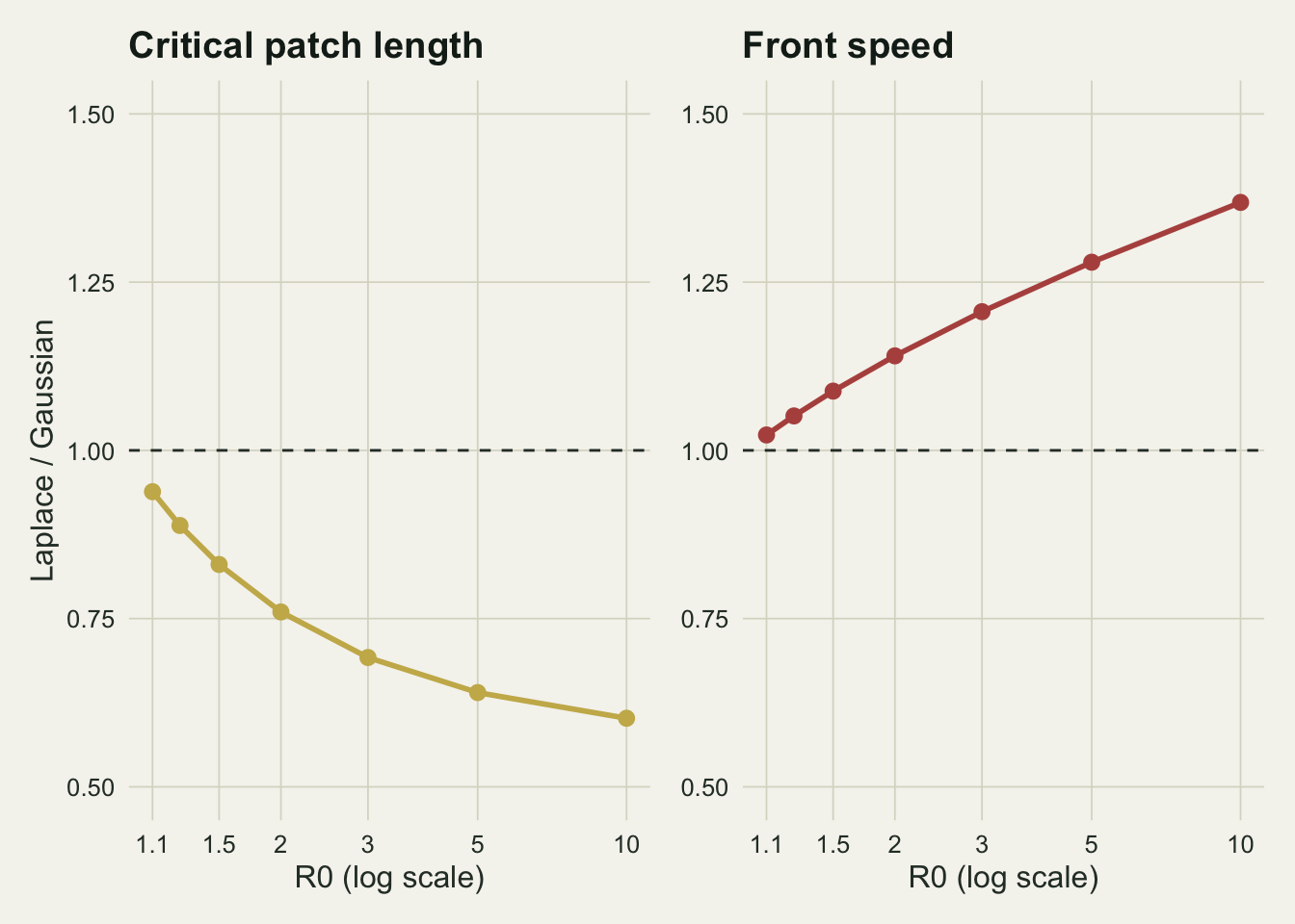
Demographic noise moves the threshold
The eigenvalue threshold belongs to a population of infinitely many individuals. A reach of margin holds a finite number of beetles, and near the threshold that number is small. The individual-based version below keeps everything the deterministic model has and adds the one thing it lacks. Each adult has a Poisson number of offspring; each offspring moves by an independent draw from the kernel; offspring landing outside the patch die. The mean offspring number is exactly \(R_0 = 1.5\) at low density, so the individual-based model and the eigenvalue calculation share the same \(R_0\) and the same kernel.
Density dependence is needed to stop populations on large patches growing without limit, and its form turns out to matter. Two versions are run. A ceiling keeps at most \(K L\) individuals, removing the excess at random after dispersal. A Beverton-Holt rule lowers the mean offspring number to \(R_0/(1 + (R_0 - 1)N/(KL))\), where \(N\) is the patch population; without edge losses its equilibrium is also \(KL\). Here \(K\) is the carrying capacity per dispersal standard deviation of habitat, set at two values. The design constants were fixed before the simulation ran: a hundred generations, the patch lengths below, and the replicate number.
n_gen   <- 100
n_rep   <- 200
k_dens  <- c(5, 20)
ibm_len <- seq(1.5, 6, by = 0.25)

draw_kern <- function(n_off, kern) {
  if (kern == "Gaussian") rnorm(n_off, 0, sd_disp)
  else rexp(n_off, alpha_lap) * (2 * (runif(n_off) < 0.5) - 1)
}

run_ibm <- function(kern, k_per_len, dd_form) {
  cell_len <- rep(ibm_len, each = n_rep)
  n_run    <- length(cell_len)
  cap      <- round(k_per_len * cell_len)
  run_id   <- rep(seq_len(n_run), cap)
  pos      <- runif(length(run_id)) * cell_len[run_id]
  for (gen in seq_len(n_gen)) {
    size_now <- tabulate(run_id, n_run)
    mu_off <- if (dd_form == "ceiling") r0_main else
      (r0_main / (1 + (r0_main - 1) * size_now / cap))[run_id]
    n_off  <- rpois(length(run_id), mu_off)
    run_id <- rep(run_id, n_off)
    pos    <- rep(pos, n_off) + draw_kern(length(run_id), kern)
    inside <- pos > 0 & pos < cell_len[run_id]
    run_id <- run_id[inside]; pos <- pos[inside]
    if (dd_form == "ceiling") {
      size_now <- tabulate(run_id, n_run)
      if (any(size_now > cap)) {
        ord    <- order(run_id, runif(length(run_id)))
        run_id <- run_id[ord]; pos <- pos[ord]
        rank_in <- seq_along(run_id) - cumsum(c(0, size_now))[run_id]
        keep   <- rank_in <= cap[run_id]
        run_id <- run_id[keep]; pos <- pos[keep]
      }
    }
    if (length(run_id) == 0) break
  }
  data.frame(kern = kern, k_dens = k_per_len, dd_form = dd_form,
             len = cell_len, alive = tabulate(run_id, n_run) > 0)
}

set.seed(6211)
ibm_runs <- do.call(rbind, lapply(c("Beverton-Holt", "ceiling"), function(dd)
  do.call(rbind, lapply(k_dens, function(kk)
    do.call(rbind, lapply(c("Gaussian", "Laplace"), function(ke) run_ibm(ke, kk, dd)))))))

persist_df <- aggregate(alive ~ kern + k_dens + dd_form + len, data = ibm_runs, FUN = mean)
persist_df$se <- sqrt(persist_df$alive * (1 - persist_df$alive) / n_rep)
mc_se_max <- sqrt(0.25 / n_rep)
half_len <- function(p_alive) {
i_up <- which(p_alive >= 0.5)[1]
if (is.na(i_up) || i_up == 1) return(NA_real_)
approx(p_alive[(i_up - 1):i_up], ibm_len[(i_up - 1):i_up], xout = 0.5)$y
}
n_boot <- 500
fit_l50 <- function(sub_runs) {
p_hat <- tapply(sub_runs$alive, sub_runs$len, mean)
boot_l <- replicate(n_boot, half_len(rbinom(length(p_hat), n_rep, p_hat) / n_rep))
c(l50 = half_len(p_hat), se = sd(boot_l, na.rm = TRUE))
}
set.seed(8093)
cell_keys <- unique(ibm_runs[, c("kern", "k_dens", "dd_form")])
l50_tab <- cbind(cell_keys, t(vapply(seq_len(nrow(cell_keys)), function(i) {
sub_runs <- ibm_runs[ibm_runs$kern == cell_keys$kern[i] &
ibm_runs$k_dens == cell_keys$k_dens[i] &
ibm_runs$dd_form == cell_keys$dd_form[i], ]
fit_l50(sub_runs)
}, numeric(2))))
l50_tab$lstar <- ifelse(l50_tab$kern == "Gaussian", lstar_gau, lstar_lap)
l50_tab$lift <- l50_tab$l50 / l50_tab$lstar
pick <- function(ke, kk, dd, col) l50_tab[l50_tab$kern == ke & l50_tab$k_dens == kk &
l50_tab$dd_form == dd, col]
bh20_gau <- pick("Gaussian", 20, "Beverton-Holt", "l50"); bh20_gau_se <- pick("Gaussian", 20, "Beverton-Holt", "se")
bh20_lap <- pick("Laplace", 20, "Beverton-Holt", "l50"); bh20_lap_se <- pick("Laplace", 20, "Beverton-Holt", "se")
bh5_gau <- pick("Gaussian", 5, "Beverton-Holt", "l50"); bh5_gau_se <- pick("Gaussian", 5, "Beverton-Holt", "se")
bh5_lap <- pick("Laplace", 5, "Beverton-Holt", "l50"); bh5_lap_se <- pick("Laplace", 5, "Beverton-Holt", "se")
cl20_gau <- pick("Gaussian", 20, "ceiling", "l50")
cl20_lap <- pick("Laplace", 20, "ceiling", "l50")
cl5_gau <- pick("Gaussian", 5, "ceiling", "l50")
cl5_lap <- pick("Laplace", 5, "ceiling", "l50")
gap_det <- lstar_gau - lstar_lap
gap_bh20 <- bh20_gau - bh20_lap
gap_bh5 <- bh5_gau - bh5_lap
gap_bh5_se <- sqrt(bh5_gau_se^2 + bh5_lap_se^2)
lift_bh20_gau <- bh20_gau / lstar_gau
lift_bh5_gau <- bh5_gau / lstar_gau
lift_cl20_gau <- cl20_gau / lstar_gau
lift_cl5_gau <- cl5_gau / lstar_gau
# deterministic Beverton-Holt equilibrium at a patch length: K L (R0 lambda - 1) / (R0 - 1)
eq_size <- function(kern, len, kk) kk * len * (r0_main * lambda_max(len, kern, n_main) - 1) / (r0_main - 1)
eq_bh20_gau <- eq_size("Gaussian", bh20_gau, 20)
eq_bh5_gau <- eq_size("Gaussian", bh5_gau, 5)
below_len <- max(ibm_len[ibm_len < lstar_gau])
below_p <- persist_df$alive[persist_df$kern == "Gaussian" & persist_df$k_dens == 20 &
persist_df$dd_form == "ceiling" & persist_df$len == below_len]
below_grow <- r0_main * lambda_max(below_len, "Gaussian", n_main)The replication was fixed at 200 runs per patch length, which puts the Monte Carlo standard error of any persistence probability at no more than 0.035. The practical threshold reported here is the patch length at which half the runs are still alive after 100 generations, read by linear interpolation between the two patch lengths either side of one half. Its standard error comes from 500 parametric bootstrap redraws of every persistence proportion from its binomial distribution. That standard error covers Monte Carlo error only. It leaves out the error of the straight line drawn across the 0.25 gap between neighbouring patch lengths, so on a curved stretch of the persistence curve the true half-persistence length can sit further from the estimate than the standard error suggests.
Under Beverton-Holt density dependence with 20 individuals of capacity per standard deviation, the half-persistence length is 3.10 (standard error 0.02) for the Gaussian kernel and 2.83 (0.02) for the Laplace. The Gaussian value is 1.35 times the deterministic critical length. With 5 per standard deviation the thresholds are 4.75 (0.05) and 4.49 (0.05), and the Gaussian lift is 2.06.
The kernel gap shrinks under the noise but does not close. Deterministically the Laplace kernel saves 0.39 standard deviations of patch. At the higher capacity the practical saving is 0.27; at the lower one it is 0.26, with a standard error of 0.07.
The ceiling tells a different story. With the same capacities the half-persistence lengths are 2.35 and 1.96 at 20 per standard deviation, and 2.96 and 2.67 at 5. The Gaussian lift is 1.02 at the higher capacity and 1.29 at the lower.
The difference between the two rules has a closed-form explanation. Patch-wide Beverton-Holt density dependence scales every individual’s offspring by the same factor, so the equilibrium keeps the shape of the dominant eigenfunction and its size solves \(R_0\lambda/(1 + (R_0-1)N/(KL)) = 1\), giving \(N^* = KL(R_0\lambda - 1)/(R_0 - 1)\). The equilibrium population shrinks to zero as the patch approaches the critical length, so a patch just above \(L^*\) promises almost no population. At the Gaussian half-persistence length the deterministic equilibrium is 18.0 individuals for the higher capacity and 14.4 for the lower: at both capacities, half the runs are lost where the deterministic model promises a population of that order. A lower capacity only means a longer patch is needed to reach it. A ceiling has no such approach: any patch above \(L^*\) fills to \(KL\), so the population that meets the noise is as large as the patch allows. The ceiling result has a catch of its own. A patch of 2.25, just below the Gaussian critical length, has a growth factor of 0.9882 per generation, and 0.220 of its ceiling runs at the higher capacity were still alive after 100 generations. Decline that slow does not finish inside the horizon, so near \(L^*\) the persistence curve measures the horizon as much as the threshold.
persist_df$panel <- factor(paste0(persist_df$dd_form, ", K = ", persist_df$k_dens),
                           levels = c("Beverton-Holt, K = 20", "Beverton-Holt, K = 5",
                                      "ceiling, K = 20", "ceiling, K = 5"))
vline_df <- data.frame(kern = c("Gaussian", "Laplace"), len = c(lstar_gau, lstar_lap))
ggplot(persist_df, aes(len, alive, colour = kern)) +
  geom_vline(data = vline_df, aes(xintercept = len, colour = kern),
             linetype = "dashed", linewidth = 0.6, show.legend = FALSE) +
  geom_errorbar(aes(ymin = alive - 1.96 * se, ymax = alive + 1.96 * se),
                width = 0.08, linewidth = 0.4, show.legend = FALSE) +
  geom_line(linewidth = 0.9) +
  geom_point(size = 1.6) +
  facet_wrap(~panel, ncol = 2) +
  scale_colour_manual(values = c(Gaussian = te_forest, Laplace = te_gold), name = NULL) +
  labs(x = "patch length (dispersal standard deviations)",
       y = "share of runs alive after 100 generations",
       title = "The practical threshold depends on density dependence",
       subtitle = "200 runs per point; bars: 95 per cent Monte Carlo intervals") +
  theme_datasheet() +
  theme(legend.position = "bottom",
        strip.text = element_text(colour = te_ink, face = "bold"))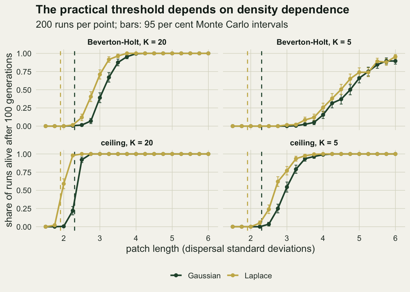
What to report
Give the critical length together with the kernel family it was computed for, and give it in units of the dispersal standard deviation as well as in metres. On the patch at \(R_0 = 1.5\) the two kernels here differ by 17 per cent at identical variance, and the difference grows with the growth rate. A variance, a mean dispersal distance or a diffusion coefficient on its own does not fix the answer.
Do not use the diffusion formula as a conservative stand-in for a species that reproduces and then disperses once a generation. For both kernels measured here it overstated the threshold, by a factor of 1.52 for the Gaussian. That factor depends on how the per-generation \(R_0\) is turned into a continuous growth rate: with \(r = \log R_0\) as here the diffusion threshold is 3.489, and with \(r = R_0 - 1\) it is 3.142, an overstatement by a factor of 1.37. If the formula is quoted, quote it as the continuous-time model it is.
Report the deterministic critical length as a lower limit, never as a design target. Under the smooth density dependence used here, half of the populations on a patch 1.35 times the critical length were gone within 100 generations at the higher capacity, and at the lower capacity the factor was 2.06. The quantity to carry into a management question is the population the patch is expected to hold, \(KL(R_0\lambda - 1)/(R_0 - 1)\) in the patch-wide Beverton-Holt case, rather than the length at which the growth factor crosses one.
State how density dependence was modelled. The same kernel, growth rate and capacity gave a practical threshold close to \(L^*\) under a ceiling at the higher capacity and well above it under Beverton-Holt. The ceiling figure carries the horizon caveat from above: 0.220 of those runs were still alive at 2.25, below \(L^*\), after 100 generations, so a longer horizon would push that threshold up. Without the rule stated, a persistence estimate from an individual-based model cannot be compared with another.
Honest limits
The patch is one-dimensional with lethal surroundings on both sides. That suits a riverbank margin, a hedgerow or a stream reach, and it is the geometry for which the Laplace closed form exists. Two-dimensional patches have a perimeter that scales differently with area, and the surroundings of most real patches are hostile rather than lethal. Van Kirk and Lewis (1997) treat fragmented habitat in which the matrix has its own growth rate below replacement, and approximate persistence from the average dispersal success of the patch; nothing here tests that case, and the Laplace-before-Gaussian ranking was not checked under it.
Only two kernel shapes are compared, both with finite moment generating functions. The loss curve suggests the peaked shape is what matters near the threshold, but a fat-tailed kernel with the same variance, or a kernel matched on the median rather than the variance as in the accelerating spread post, could order differently, and matching on a different moment changes every ratio reported above.
Density dependence in the individual-based model acts on the whole patch at once. An adult near the edge is held back by crowding in the middle, which no animal experiences. Local crowding would hold back the crowded centre of the patch more than its thinner edges and change the shape of the population the noise acts on. Neither the size nor the direction of that effect on the practical threshold was measured here.
The horizon of 100 generations and the start at capacity are design choices, and the persistence curves depend on both. Near the critical length the decline is so slow that a longer horizon would lower every persistence curve there, as the ceiling runs just below \(L^*\) showed. There is no environmental stochasticity at all. Bad years hitting the whole patch together would be expected to raise the practical threshold further and would do so without any reference to the kernel.
Finally, the model has one life stage, a fixed per-capita \(R_0\) and no Allee effect. A mate-finding Allee effect would make a small population on a marginal patch decline faster than any of the models here, and that situation belongs to Allee effects and extinction risk rather than to this post.
References
Skellam JG 1951 Biometrika 38(1-2):196-218 (10.1093/biomet/38.1-2.196)
Kot M, Schaffer WM 1986 Mathematical Biosciences 80(1):109-136 (10.1016/0025-5564(86)90069-6)
Weinberger HF 1982 SIAM Journal on Mathematical Analysis 13(3):353-396 (10.1137/0513028)
Van Kirk RW, Lewis MA 1997 Bulletin of Mathematical Biology 59(1):107-137 (10.1007/BF02459473)