library(ggplot2)
library(patchwork)
library(splines)
library(mgcv)

te_paper  <- "#f5f4ee"
te_ink    <- "#16241d"
te_body   <- "#2c3a31"
te_forest <- "#275139"
te_rust   <- "#b5534e"
te_gold   <- "#c9b458"
te_line   <- "#dad9ca"

theme_datasheet <- function() {
  theme_minimal(base_size = 12) +
    theme(plot.background  = element_rect(fill = te_paper, colour = NA),
          panel.background = element_rect(fill = te_paper, colour = NA),
          panel.grid.major = element_line(colour = te_line, linewidth = 0.3),
          panel.grid.minor = element_blank(),
          text             = element_text(colour = te_body),
          plot.title       = element_text(colour = te_ink, face = "bold"),
          plot.subtitle    = element_text(colour = te_body),
          axis.text        = element_text(colour = te_body))
}Habitat amount versus fragmentation per se
R
landscape ecology
fragmentation
GLM
simulation
ecology tutorial
A bird tracking only forest amount gains a false edge density effect once amount enters a GLM as a straight line. Measuring in R which model or design fixes it.
A regional atlas has breeding pair counts of a woodland bird from square landscapes of four by four kilometres, and each landscape has a forest map. The question the study was funded for is the one Fahrig 2003 set out for the whole field: once the amount of forest is accounted for, does the way it is broken up matter as well? Fragmentation per se, in her sense, is the breaking apart of habitat independent of how much of it there is, and it is usually measured with configuration metrics such as the number or density of patches and the amount of edge. The standard analysis is a Poisson regression of the count on forest amount and edge density together, and the headline is the edge density coefficient.
The mechanism that can make that coefficient lie is already measured on this site, in a different setting. The section on the ANCOVA line with the wrong shape fits a straight line to a curved relation between liver mass and body mass and shows the wrong shape leaking into the site term: the slide to a common body size “is wrong by an amount that depends on how far it has to go”, and the false positive rate climbs with the size gap. Here the curved covariate is forest amount and the correlated term is a configuration metric. The post on collinearity and VIF is the other half of the usual advice: correlated predictors in one correctly specified model inflate the standard errors and hide a real effect, which is a loss of precision and not a bias. What follows is about bias.
Patch metrics and fragmentation supplies the machinery used below (a smoothed noise landscape generator and a label propagation patch counter) and shows that edge density and patch count change enormously at a fixed habitat amount, but it has no response variable and never samples landscapes. None of the result is new. Koper, Schmiegelow and Merrill 2007 showed that residualising a fragmentation index on habitat amount cannot separate the two effects, Smith and colleagues 2009 compared the statistical methods ecologists use to separate the effects of habitat loss and fragmentation, and Pasher and colleagues 2013 proposed choosing study landscapes so that the landscape variables are uncorrelated. This post is a demonstration of those arguments with one species whose true response contains no configuration term at all, and it adds one measurement the design advice needs: which correlation the landscape selection has to remove.
A pool of landscapes and a species that counts forest
Every landscape is a 40 by 40 grid of 100 m cells. Uniform noise is smoothed between zero and eight times, which sets how clumped the forest is, and then thresholded so that the forest amount is a draw between 5 and 60 per cent. Edge density is the number of forest to non-forest cell sides, in metres of edge per hectare; patch density is the number of four-connected forest patches per 100 ha, counted by label propagation. The pool of 1500 landscapes plays the part of the region a study could sample from.
side <- 40; n_pool <- 1500; max_pass <- 8     # 40 x 40 cells of 100 m
amount_lo <- 0.05; amount_hi <- 0.6
k_max <- 20; a_half <- 0.15                    # the species: pairs at saturation, half-scale

smooth_once <- function(z) {
  n <- nrow(z)
  (z + rbind(z[1, ], z[-n, ]) + rbind(z[-1, ], z[n, ]) +
     cbind(z[, 1], z[, -n]) + cbind(z[, -1], z[, n])) / 5
}

count_patches <- function(hab) {
  n <- nrow(hab); lab <- matrix(0L, n, n); lab[hab] <- seq_len(sum(hab))
  repeat {
    old <- lab
    best <- pmax(lab, rbind(0L, lab[-n, ]), rbind(lab[-1, ], 0L),
                 cbind(0L, lab[, -n]), cbind(lab[, -1], 0L))
    lab[hab] <- best[hab]
    if (identical(lab, old)) break
  }
  length(unique(lab[hab]))
}

make_landscape <- function() {
  passes <- sample(0:max_pass, 1)
  z <- matrix(runif(side * side), side)
  for (i in seq_len(passes)) z <- smooth_once(z)
  hab <- z > quantile(z, 1 - runif(1, amount_lo, amount_hi))
  edges <- sum(hab[-1, ] != hab[-side, ]) + sum(hab[, -1] != hab[, -side])
  c(amount = mean(hab), ed = 100 * edges / side^2,
    pd = 100 * count_patches(hab) / side^2, passes = passes)
}

set.seed(4711)
pool <- as.data.frame(t(replicate(n_pool, make_landscape())))
mean_pairs <- function(amount) k_max * (1 - exp(-amount / a_half))

cor_ed <- cor(pool$amount, pool$ed); cor_pd <- cor(pool$amount, pool$pd)
cor_ed_pd <- cor(pool$ed, pool$pd)
ed_rng <- range(pool$ed)
straight <- lm(log(mean_pairs(amount)) ~ amount, data = pool)
share_30 <- mean_pairs(0.3) / mean_pairs(amount_hi)
curve_gap <- range(resid(straight))
curv_pool_q <- resid(lm(I(amount^2) ~ amount, data = pool))   # amount squared minus its straight-line part
curv_cor_ed <- cor(curv_pool_q, pool$ed); curv_cor_pd <- cor(curv_pool_q, pool$pd)
quad_coef <- sapply(split(pool, pool$passes), function(d)
  c(ed = coef(lm(ed ~ amount + I(amount^2), data = d))[3],
    pd = coef(lm(pd ~ amount + I(amount^2), data = d))[3]))
n_neg_ed <- sum(quad_coef[1, ] < 0); n_neg_pd <- sum(quad_coef[2, ] < 0)
Across the pool, edge density runs from 5.6 to 101.0 m per ha and its correlation with forest amount is 0.45. Patch density has a correlation of -0.09 with amount, of the opposite sign, and 0.77 with edge density. Both metrics bend: edge density rises steeply with amount at low cover and flattens at high cover, and patch density rises and then falls. Fitted with a quadratic in amount within each of the 9 smoothing levels, the squared term is negative in 9 levels for edge density and 9 for patch density. Across the pool, the correlation with the curvature of amount (amount squared with its straight-line part removed) is -0.17 for edge density and -0.20 for patch density. The two do not share the sign of their linear relation to amount, which becomes useful later.
The species responds to forest amount and nothing else. The expected number of pairs is 20 times one minus the exponential of minus amount over 0.15, which saturates: a landscape with 30 per cent forest already holds 88 per cent of the pairs expected at 60 per cent. On the log scale of a Poisson model that curve is concave, and a straight line in amount misses it by between -0.58 and +0.15 log units across the pool.
a_seq <- seq(amount_lo, amount_hi, length.out = 200)
curve_df <- data.frame(amount = a_seq, truth = log(mean_pairs(a_seq)),
                       line = predict(straight, newdata = data.frame(amount = a_seq)))
p_curve <- ggplot(curve_df, aes(amount)) +
  geom_line(aes(y = line), colour = te_rust, linewidth = 0.8, linetype = "dashed") +
  geom_line(aes(y = truth), colour = te_forest, linewidth = 1) +
  labs(x = "forest amount", y = "log expected pairs", title = "The response",
       subtitle = "dashed: straight line") +
  theme_datasheet()
p_ed <- ggplot(pool, aes(amount, ed)) +
  geom_point(colour = te_forest, alpha = 0.25, size = 0.8) +
  labs(x = "forest amount", y = "edge density (m per ha)", title = "Edge density",
       subtitle = sprintf("correlation with amount %.2f", cor_ed)) +
  theme_datasheet()
p_pd <- ggplot(pool, aes(amount, pd)) +
  geom_point(colour = te_gold, alpha = 0.35, size = 0.8) +
  labs(x = "forest amount", y = "patches per 100 ha", title = "Patch density",
       subtitle = sprintf("correlation with amount %.2f", cor_pd)) +
  theme_datasheet()
p_curve + p_ed + p_pd + plot_annotation(theme = theme_datasheet())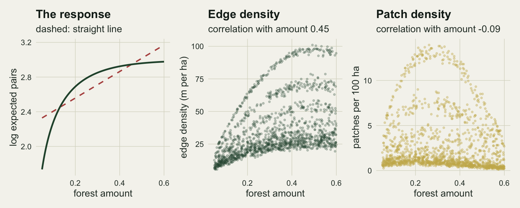
A fragmentation effect that is not there
A study draws m landscapes at random from the pool, counts the pairs in each, and fits three Poisson regressions that all contain the configuration metric: one with forest amount as a straight line, one with log amount, and one with a natural cubic spline in amount on four degrees of freedom. The spline was fixed at four degrees of freedom before anything was run. Each study is analysed twice, once with edge density and once with patch density as the configuration term, on the same counts. The rate of p < 0.05 for the configuration term is a false positive rate, because the truth has no configuration term.
fit_last <- function(X, y) {          # Poisson GLM, Wald test of the last column
  f  <- glm.fit(X, y, family = poisson())
  k  <- ncol(X); b <- f$coefficients[k]
  se <- sqrt(chol2inv(qr.R(f$qr))[k, k])
  c(b, 2 * pnorm(-abs(b / se)))
}

study_fits <- function(idx) {
  a <- pool$amount[idx]; e <- pool$ed[idx]; p <- pool$pd[idx]
  y <- rpois(length(idx), mean_pairs(a)); B <- ns(a, df = 4)
  c(fit_last(cbind(1, a, e), y), fit_last(cbind(1, log(a), e), y), fit_last(cbind(1, B, e), y),
    fit_last(cbind(1, a, p), y), fit_last(cbind(1, log(a), p), y), fit_last(cbind(1, B, p), y))
}

m_grid <- c(24, 48, 100, 150); n_study <- 2000
form_lev <- c("straight line", "log amount", "spline")
set.seed(918)
sweep_raw <- lapply(m_grid, function(m) t(replicate(n_study, study_fits(sample.int(n_pool, m)))))

sw_tab <- do.call(rbind, lapply(seq_along(m_grid), function(j) {
  s <- sweep_raw[[j]]
  data.frame(m = m_grid[j],
             metric = rep(c("edge density", "patch density"), each = 3),
             form = factor(rep(form_lev, 2), levels = form_lev),
             rate = colMeans(s[, seq(2, 12, 2)] < 0.05),
             pos = c(sapply(seq(1, 11, 2), function(k) mean(s[s[, k + 1] < 0.05, k] > 0))))
}))
sw_tab$mcse <- sqrt(sw_tab$rate * (1 - sw_tab$rate) / n_study)
rt <- function(m, metric, k) sw_tab$rate[sw_tab$m == m & sw_tab$metric == metric & sw_tab$form == form_lev[k]]
ps <- function(m, metric) sw_tab$pos[sw_tab$m == m & sw_tab$metric == metric & sw_tab$form == form_lev[1]]
mcse_05 <- sqrt(0.05 * 0.95 / n_study)
spl_rates <- sw_tab$rate[sw_tab$form == form_lev[3]]
With the straight line, edge density comes out significant in 8.9 per cent of studies of 24 landscapes, 10.8 per cent at 48, 16.4 per cent at 100 and 18.8 per cent at 150. The false effect is not random in direction: at 150 landscapes 99 per cent of the significant edge density coefficients are positive, so the study reports that a more fragmented landscape with the same forest amount holds more pairs. Patch density behaves the same way, 11.5 per cent at 48 landscapes and 23.3 per cent at 150, with 99.8 per cent of the significant coefficients positive, even though patch density is negatively correlated with amount. The sign of a metric’s linear correlation with amount does not set the sign of the leak. What sets it is the bend: the log response is concave in amount, both metrics are concave in amount too (the negative curvature correlations above), so whatever the straight line leaves unexplained is picked up by the configuration term with a positive sign. That point returns in the design section.
The spline removes the rate. Across all eight combinations of study size and metric it stays between 4.3 and 5.7 per cent, against a Monte Carlo standard error of 0.5 percentage points at five per cent. Log amount is a better guess than a straight line, but it is also the wrong curve: with edge density it gives 6.0 per cent at 150 landscapes, and with patch density 10.5 per cent.
ggplot(sw_tab, aes(m, rate, colour = form)) +
  geom_hline(yintercept = 0.05, colour = te_body, linetype = "dashed", linewidth = 0.5) +
  geom_errorbar(aes(ymin = rate - 2 * mcse, ymax = rate + 2 * mcse), width = 4, linewidth = 0.4) +
  geom_line(linewidth = 0.9) + geom_point(size = 2) +
  facet_wrap(~metric) +
  scale_colour_manual(values = c(te_rust, te_gold, te_forest), name = "amount term") +
  scale_x_continuous(breaks = m_grid) +
  scale_y_continuous(limits = c(0, NA)) +
  labs(x = "landscapes in the study", y = "rate of p < 0.05, no true effect",
       title = "The straight line leaks into configuration",
       subtitle = "dashed line: the nominal five per cent") +
  theme_datasheet() + theme(legend.position = "bottom")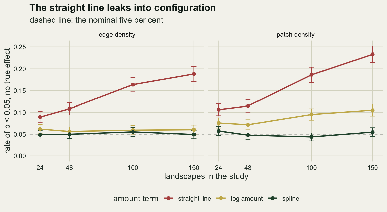
The rate grows with study size for the reason given in the ANCOVA post: the bias in the coefficient does not shrink as landscapes are added, and its standard error does. A larger study is a more reliable detector of the wrong model.
The check with a penalised smooth, as most people would fit it, uses mgcv on a smaller set of studies at the largest size.
n_gam <- 300
set.seed(8150)
p_gam <- replicate(n_gam, {
  idx <- sample.int(n_pool, 150)
  d <- data.frame(amount = pool$amount[idx], ed = pool$ed[idx])
  d$y <- rpois(150, mean_pairs(d$amount))
  summary(gam(y ~ s(amount) + ed, family = poisson, data = d, method = "REML"))$p.table["ed", 4]
})
gam_rate <- mean(p_gam < 0.05); gam_mcse <- sqrt(gam_rate * (1 - gam_rate) / n_gam)
Over 300 studies of 150 landscapes, gam(y ~ s(amount) + ed) with REML smoothness selection gives an edge density rate of 5.0 per cent, with a Monte Carlo standard error of 1.3 points.
Residuals: the credit and the curvature
The most common repair in the per se literature is the one Koper and colleagues 2007 examined: regress the fragmentation index on habitat amount and use the residual as the fragmentation variable. The post on residuals as a variable shows, through the Frisch-Waugh-Lovell theorem, that in a linear model a residualised predictor returns exactly the coefficient of the one model, and prices the interval that the two-step then prints. Here the model is a Poisson GLM with amount kept next to the residual, and the same projection argument still makes the coefficient identical, as the chunk below checks. What this section adds is a residual taken on a curved fit of amount rather than a straight line.
n_res <- 2000
set.seed(6150)
res_raw <- t(replicate(n_res, {
  idx <- sample.int(n_pool, 150)
  a <- pool$amount[idx]; e <- pool$ed[idx]; y <- rpois(150, mean_pairs(a))
  e_res <- resid(lm(e ~ a)); a_res <- resid(lm(a ~ e))
  e_res_quad <- resid(lm(e ~ a + I(a^2))); e_res_ns <- resid(lm(e ~ ns(a, df = 4)))
  c(fit_last(cbind(1, a, e), y),            # both raw
    fit_last(cbind(1, a, e_res), y),        # edge density residualised on amount
    fit_last(cbind(1, a_res, e), y),        # amount residualised on edge density
    fit_last(cbind(1, a, e_res_quad), y),   # residualised on a quadratic, straight line kept
    fit_last(cbind(1, a, e_res_ns), y))     # residualised on a spline, straight line kept
}))
res_gap  <- max(abs(res_raw[, 1] - res_raw[, 3]))
res_rate <- colMeans(res_raw[, c(2, 4, 6, 8, 10)] < 0.05)
res_mcse <- sqrt(res_rate * (1 - res_rate) / n_res)
Residualising edge density on amount leaves the edge density coefficient exactly where it was. The largest difference from the plain model over 2000 studies is 3.1e-17, which is rounding, and the false positive rates are 17.3 and 17.3 per cent. This is algebra, not luck (the same projection argument as in that post): the residual is edge density minus a straight line in amount, and amount is already in the model, so the new design matrix spans the same space and only the amount coefficient changes. A residual from a straight-line regression on amount cannot fix a leak that comes through the shape of the amount term. A residual from a curved fit can: residualising edge density on a quadratic in amount, with the straight line still in the model, gives 4.7 per cent, and on a spline with four degrees of freedom 4.6 per cent (Monte Carlo standard errors near 0.5 points). That works because the curvature of amount is taken out of the configuration variable instead of being put into the model; a spline in amount does the same job openly, and keeps the amount term a description of the species. Reverse the order, residualise amount on edge density instead, and the edge density coefficient absorbs everything amount and edge density share: the configuration term is then significant in 99.9 per cent of studies. That is what Koper and colleagues found with prairie songbirds: which variable is residualised decides which one gets the credit, and the data have no say in it.
Choosing landscapes: which correlation matters
Pasher and colleagues 2013 recommend selecting study landscapes so that the landscape variables span their range and are uncorrelated, and the idea is sound. The question for this species is which correlation the selection has to remove. Five designs of 150 landscapes are compared. The first is the random draw used so far. The second is a grid in the ranks of amount and edge density, one landscape per occupied cell, topped up at random to 150 when fewer cells are occupied. The last three take one landscape per amount stratum and then swap landscapes within strata until a target is met: a correlation of 0.2 between amount and edge density, a correlation of zero, or a correlation of zero between edge density and the curvature of amount, which is amount squared with its straight-line part removed (that term is convex, so a metric that bends like the concave response correlates with it negatively). The curvature target uses only the landscape variables, so an analyst can compute it without knowing the response. For every selected set the post records both correlations as achieved, not as targeted.
m_des <- 150; n_des <- 1000
strata  <- cut(pool$amount, quantile(pool$amount, 0:m_des / m_des),
               include.lowest = TRUE, labels = FALSE)
members <- split(seq_len(n_pool), strata)
curv_pool <- resid(lm(I(amount^2) ~ amount, data = pool))

pick_random <- function() sample.int(n_pool, m_des)

pick_grid <- function() {
  k <- ceiling(sqrt(m_des))
  cell <- interaction(cut(rank(pool$amount), k, labels = FALSE),
                      cut(rank(pool$ed), k, labels = FALSE), drop = TRUE)
  idx <- vapply(split(seq_len(n_pool), cell), function(v) v[sample.int(length(v), 1)], 1L)
  idx <- idx[sample.int(length(idx))]
  if (length(idx) < m_des) idx <- c(idx, sample(setdiff(seq_len(n_pool), idx), m_des - length(idx)))
  idx[seq_len(m_des)]
}

pick_swap <- function(partner, target, n_try = 60 * m_des, tol = 0.005) {
  idx <- vapply(members, function(v) v[sample.int(length(v), 1)], 1L)
  w <- partner; e <- pool$ed; m <- m_des
  s <- c(sum(w[idx]), sum(e[idx]), sum(w[idx]^2), sum(e[idx]^2), sum(w[idx] * e[idx]))
  r_of <- function(s) (s[5] - s[1] * s[2] / m) / sqrt((s[3] - s[1]^2 / m) * (s[4] - s[2]^2 / m))
  gap <- abs(r_of(s) - target)
  js <- sample.int(m, n_try, replace = TRUE); us <- runif(n_try)
  for (tr in seq_len(n_try)) {
    if (gap < tol) break
    j <- js[tr]; v <- members[[j]]; new <- v[ceiling(us[tr] * length(v))]; old <- idx[j]
    s_new <- s + c(w[new] - w[old], e[new] - e[old], w[new]^2 - w[old]^2,
                   e[new]^2 - e[old]^2, w[new] * e[new] - w[old] * e[old])
    g_new <- abs(r_of(s_new) - target)
    if (g_new < gap) { idx[j] <- new; s <- s_new; gap <- g_new }
  }
  idx
}

design_fits <- function(idx) {
  a <- pool$amount[idx]; e <- pool$ed[idx]; y <- rpois(length(idx), mean_pairs(a))
  c(cor(a, e), cor(resid(lm(I(a^2) ~ a)), e),
    fit_last(cbind(1, a, e), y)[2], fit_last(cbind(1, ns(a, df = 4), e), y)[2],
    tapply(e, cut(a, c(0, 0.2, 0.4, 1)), mean),
    fit_last(cbind(1, a, a^2, e), y)[2],                 # quadratic in amount
    cor(resid(lm(log(mean_pairs(a)) ~ a)), e),           # what the straight line misses, true response
    sd(resid(lm(log(mean_pairs(a)) ~ a))),               # spread of that missed part
    cor(resid(lm(log(mean_pairs(a)) ~ a + I(a^2))), e))  # what a quadratic still misses
}

des_lev <- c("random draw", "rank grid", "amount cor 0.2", "amount cor 0", "curvature cor 0")
pickers <- list(pick_random, pick_grid,
                function() pick_swap(pool$amount, 0.2), function() pick_swap(pool$amount, 0),
                function() pick_swap(curv_pool, 0))
set.seed(5150)
des_raw <- lapply(pickers, function(f) t(replicate(n_des, design_fits(f()))))
des_tab <- data.frame(design = factor(des_lev, levels = des_lev),
  cor_amount = sapply(des_raw, function(d) mean(d[, 1])),
  cor_curv   = sapply(des_raw, function(d) mean(d[, 2])),
  line = sapply(des_raw, function(d) mean(d[, 3] < 0.05)),
  spline = sapply(des_raw, function(d) mean(d[, 4] < 0.05)),
  quad   = sapply(des_raw, function(d) mean(d[, 8] < 0.05)),
  cor_miss = sapply(des_raw, function(d) mean(d[, 9])),
  sd_miss  = sapply(des_raw, function(d) mean(d[, 10])),
  cor_miss_q = sapply(des_raw, function(d) mean(d[, 11])))
des_tab$mcse <- sqrt(des_tab$line * (1 - des_tab$line) / n_des)
band <- sapply(des_raw, function(d) colMeans(d[, 5:7]))   # mean edge density by amount band
dt <- function(k, col) des_tab[[col]][k]
mcse_des <- sqrt(0.05 * 0.95 / n_des)
k_grid <- ceiling(sqrt(m_des))
n_cells <- nlevels(interaction(cut(rank(pool$amount), k_grid, labels = FALSE),
                               cut(rank(pool$ed), k_grid, labels = FALSE), drop = TRUE))
round(des_tab[, -1], 3)
cor_amount cor_curv line spline quad cor_miss sd_miss cor_miss_q mcse
1 0.448 -0.175 0.191 0.050 0.054 0.162 0.145 0.010 0.012
2 0.286 -0.158 0.141 0.055 0.055 0.154 0.128 0.027 0.011
3 0.201 -0.308 0.456 0.049 0.058 0.324 0.146 0.107 0.016
4 0.001 -0.365 0.653 0.058 0.124 0.431 0.146 0.235 0.015
5 0.506 -0.003 0.059 0.055 0.059 0.025 0.146 0.051 0.007The random draw has a correlation of 0.45 between amount and edge density, a curvature correlation of -0.17, and a straight-line false positive rate of 19.1 per cent. The rank grid (13 by 13 cells, of which 138 are occupied, so 12 landscapes are random padding) lowers the amount correlation to 0.29, barely moves the curvature correlation (-0.16), and brings the rate down only to 14.1 per cent.
Swapping landscapes to push the amount correlation down makes the leak worse, not better. At an achieved correlation of 0.20 the curvature correlation is -0.31 and the rate 45.6 per cent; at 0.001, a selected set in which amount and edge density look perfectly unrelated, the curvature correlation is -0.37 and the straight-line model finds a fragmentation effect in 65.3 per cent of studies. The selected sets show why. In a random draw the mean edge density is 20.7, 37.8 and 45.7 m per ha in landscapes below 20, between 20 and 40, and above 40 per cent forest. The swaps that reach zero correlation take busier landscapes at low cover and simpler ones at high cover, giving 28.6, 43.4 and 30.7: the straight trend is gone and a hump with its peak in the middle band is left, which is exactly the shape the straight line in amount fails to fit. The last design ignores the linear correlation altogether. Its sets have an amount correlation of 0.51, higher than a random draw, a curvature correlation of -0.003, band means of 21.5, 33.3 and 47.2, and a rate of 5.9 per cent.
des_long <- rbind(
  data.frame(des_tab[, c("design", "line", "mcse")], x = des_tab$cor_amount,
             panel = "correlation with amount"),
  data.frame(des_tab[, c("design", "line", "mcse")], x = des_tab$cor_curv,
             panel = "correlation with curvature of amount"))
des_cols <- c("#8c968f", te_gold, "#8a7f3a", te_rust, te_forest)
ggplot(des_long, aes(x, line, colour = design)) +
  geom_hline(yintercept = 0.05, colour = te_body, linetype = "dashed", linewidth = 0.5) +
  geom_errorbar(aes(ymin = line - 2 * mcse, ymax = line + 2 * mcse), width = 0.015, linewidth = 0.5) +
  geom_point(size = 3) +
  facet_wrap(~panel, scales = "free_x") +
  scale_colour_manual(values = des_cols, name = NULL) +
  scale_y_continuous(limits = c(0, NA)) +
  guides(colour = guide_legend(nrow = 2)) +
  labs(x = "achieved correlation with edge density in the selected set",
       y = "rate of p < 0.05, straight-line amount",
       title = "The leak follows the curvature correlation",
       subtitle = "150 landscapes; dashed line: the nominal five per cent") +
  theme_datasheet() + theme(legend.position = "bottom")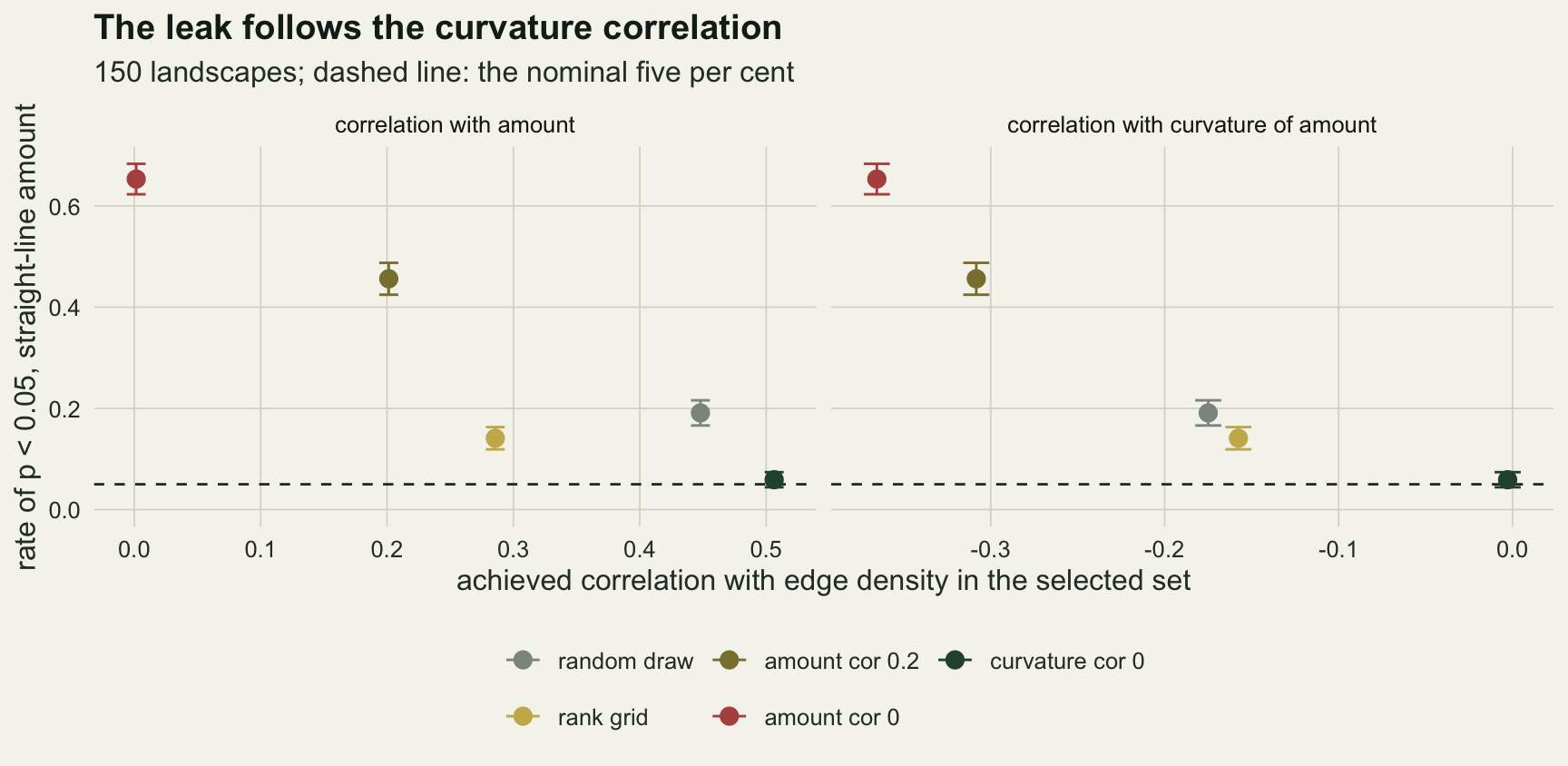
Against the linear correlation the rate mostly rises as the correlation falls, the opposite of what the design advice expects, and the rank grid breaks even that pattern. Against the curvature correlation the rate grows with the size of the correlation, with the rank grid a few points below the random draw at almost the same value.
The curvature correlation is a proxy, and the chunk also records what it stands in for. The quantity the straight-line model gets wrong is the part of the true log response that a straight line in amount misses; the edge density coefficient absorbs whatever of that part edge density can reproduce at a given amount, which is the omitted-variable bias. The correlation of edge density with that missed part is 0.16 in the random draw, 0.15 in the rank grid, 0.32 and 0.43 in the two amount-correlation swaps and 0.025 in the curvature swap, the same ordering as the rates. The size of the leak also scales with how much the missed part varies across the selected landscapes, and the rank grid has less of it: its standard deviation is 0.128 log units against 0.145 in the random draw, so at nearly the same correlation it leaks less.
The direct test of the mechanism is to put the curvature into the model. A quadratic in amount, fitted to the same selected sets, brings four of the designs to between 5.4 and 5.9 per cent. In the sets swapped to zero amount correlation, the ones pushed hardest towards the hump shape, it leaves 12.4 per cent: there a quadratic does not take up all of what the straight line misses, and edge density still has a correlation of 0.24 with the part of the true log response that a quadratic in amount misses, against 0.01 in the random draw. The spline gives between 4.9 and 5.8 per cent across all five (Monte Carlo standard error 0.7 points at five per cent), so a flexible amount term repairs whatever the design leaves, and with it the choice of design no longer matters for this test.
A real edge effect, shifted
Bias does not only create effects. A second arm gives the species a real configuration response, a change of 0.03 on the log scale per 10 m per ha of edge density, negative in one set of studies and positive in the other, on top of the same amount curve, and fits the straight line and the spline to random draws of 150 landscapes.
beta_grid <- c(-0.03, 0.03); n_real <- 2000
set.seed(7150)
real_raw <- lapply(beta_grid, function(b) t(replicate(n_real, {
  idx <- sample.int(n_pool, 150); a <- pool$amount[idx]; e <- pool$ed[idx]
  y <- rpois(150, mean_pairs(a) * exp(b * (e - mean(pool$ed)) / 10))
  c(fit_last(cbind(1, a, e), y), fit_last(cbind(1, ns(a, df = 4), e), y))
})))
real_sum <- sapply(seq_along(beta_grid), function(j) {
  r <- real_raw[[j]]; b <- beta_grid[j]
  c(line_mean = 10 * mean(r[, 1]), spline_mean = 10 * mean(r[, 3]),
    line_det = mean(r[, 2] < 0.05 & sign(r[, 1]) == sign(b)),
    spline_det = mean(r[, 4] < 0.05 & sign(r[, 3]) == sign(b)))
})
shift <- real_sum["line_mean", ] - beta_grid
truth_lev <- sprintf("true effect %+.2f", beta_grid)
real_df <- do.call(rbind, lapply(seq_along(beta_grid), function(j) rbind(
  data.frame(truth = sprintf("true effect %+.2f", beta_grid[j]), form = "straight line",
             est = 10 * real_raw[[j]][, 1]),
  data.frame(truth = sprintf("true effect %+.2f", beta_grid[j]), form = "spline",
             est = 10 * real_raw[[j]][, 3]))))
real_df$form <- factor(real_df$form, levels = c("straight line", "spline"))
real_df$truth <- factor(real_df$truth, levels = truth_lev)
With a true effect of -0.03 the straight line estimates -0.020 on average and detects the negative effect in 48.0 per cent of studies; the spline estimates -0.031 and detects it in 82.8 per cent. With a true effect of +0.03 the straight line estimates +0.039 and detects it in 98.0 per cent, against +0.030 and 86.4 per cent for the spline. The straight line moves the average estimate by +0.010 and +0.009, nearly the same shift in both directions of truth, so a harmful configuration effect is understated by about a third and about half of the studies miss it, while a beneficial one is overstated and looks easier to detect than it is.
truth_df <- data.frame(truth = factor(truth_lev, levels = truth_lev), value = beta_grid)
ggplot(real_df, aes(est, fill = form)) +
  geom_density(alpha = 0.55, colour = NA) +
  geom_vline(data = truth_df, aes(xintercept = value), colour = te_ink,
             linetype = "dashed", linewidth = 0.7) +
  facet_wrap(~truth, scales = "free_x") +
  scale_fill_manual(values = c(te_rust, te_forest), name = "amount term") +
  labs(x = "estimated effect per 10 m per ha of edge density (log scale)", y = "density",
       title = "The straight line shifts the estimates upward",
       subtitle = "dashed line: the true effect") +
  theme_datasheet() + theme(legend.position = "bottom", plot.margin = margin(6, 22, 6, 6))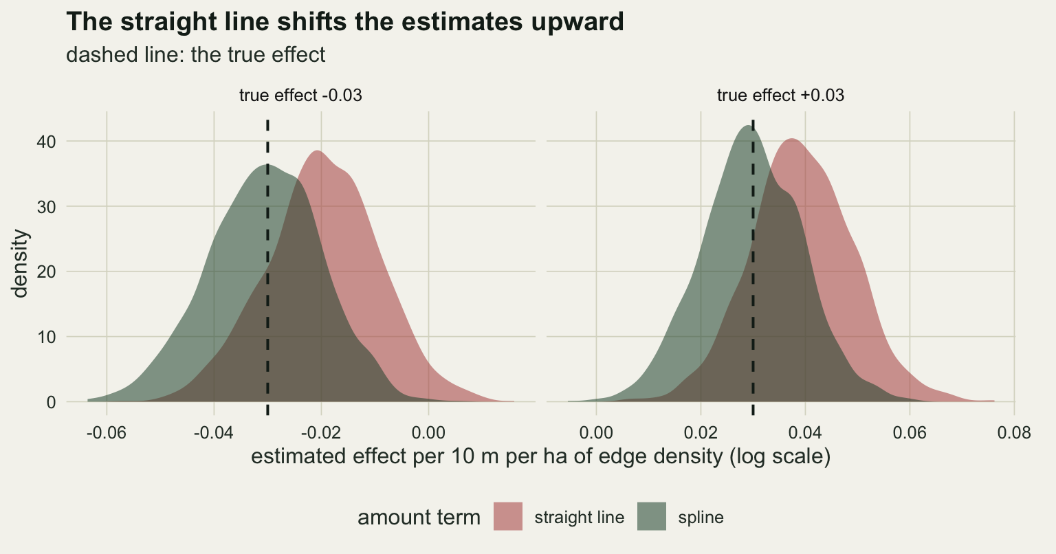
What to report
Report the form of the amount term and why it was chosen. A straight line in amount is an assumption about the species, and in this simulation it is the whole source of the fragmentation per se effect. A flexible term (a spline, or a smooth in mgcv) costs a few degrees of freedom, and with 150 landscapes there are plenty.
Report the correlation of the configuration metric with amount, and next to it the correlation with the curvature of amount, computed on the landscapes actually used. The first is the one everybody gives; the second tracked the size of the leak across the designs measured here, and the first did not.
If landscapes were selected to decorrelate amount and configuration, report the achieved correlations of the selected set, not the target. A set with zero linear correlation was the worst design above.
If the configuration effect disappears when amount is fitted flexibly, say that, and treat the straight-line estimate as a property of the model. If residuals were used, say which variable was residualised on which, because that choice decides the answer and is not a finding about the landscape.
Honest limits
Everything comes from one neutral generator. Smoothed and thresholded noise ties edge density to amount in a particular way, a concave rise in bands set by the number of smoothing passes; real forest maps, shaped by roads, fields and topography, can give a different joint distribution and a different curvature correlation. The size of the rates is a property of this pool, and the ranking of the designs is what should carry over.
The configuration effect, where there is one, is additive on the log scale and the same at every forest amount. An effect that appears only below some cover threshold, the fragmentation threshold idea, would need an amount by configuration interaction, and neither the spline nor the design comparison here tests one.
The species has one saturating response and Poisson counts with no overdispersion and no spatial autocorrelation among landscapes. A response closer to a straight line on the log scale leaks less; overdispersed counts analysed as Poisson would add false positives of their own that have nothing to do with configuration, which is why the error model here was kept exact.
The curvature correlation uses only the quadratic part of amount. The design that set it to zero brought the straight-line rate down to 5.9 per cent, not exactly to five, and a response with a sharper bend would leave more of the leak in the cubic and higher terms. Selecting on it also changes which landscapes are sampled, and nothing here checks whether the selected sets are representative of the region for other purposes.
The spline was fixed at four degrees of freedom. Its highest rate anywhere in the post is 5.8 per cent, within two Monte Carlo standard errors of five, but a response with a sharper threshold than this one could need more flexibility than four degrees of freedom give. Configuration was measured at one grain and one extent, and the patch-scale version of the question, where an edge penalty acts inside patches as in SLOSS and reserve configuration, was not simulated.
References
Fahrig L 2003 Annual Review of Ecology, Evolution, and Systematics 34:487-515 (10.1146/annurev.ecolsys.34.011802.132419)
Koper N, Schmiegelow FKA, Merrill EH 2007 Landscape Ecology 22(6):811-820 (10.1007/s10980-007-9083-9)
Smith AC, Koper N, Francis CM, Fahrig L 2009 Landscape Ecology 24(10):1271-1285 (10.1007/s10980-009-9383-3)
Pasher J, Mitchell SW, King DJ, Fahrig L, Smith AC, Lindsay KE 2013 Landscape Ecology 28(3):371-383 (10.1007/s10980-013-9852-6)