library(ggplot2)

theme_te <- function(base_size = 11) {
  theme_minimal(base_size = base_size) +
    theme(panel.grid.minor = element_blank(),
          panel.grid.major = element_line(colour = "#dad9ca", linewidth = 0.3),
          axis.title = element_text(colour = "#46604a"),
          axis.text = element_text(colour = "#5d6b61"),
          plot.title = element_text(colour = "#16241d", face = "bold"),
          plot.subtitle = element_text(colour = "#5d6b61"),
          legend.title = element_text(colour = "#46604a"),
          legend.text = element_text(colour = "#5d6b61"),
          plot.background = element_rect(fill = "#f5f4ee", colour = NA),
          panel.background = element_rect(fill = "#f5f4ee", colour = NA))
}

lam_a <- 0.9; lam_b <- 0.7
sd_a  <- 0.6; sd_b  <- 0.5

Sigma_driver <- matrix(c(lam_a^2 + sd_a^2, lam_a * lam_b,
                         lam_a * lam_b,    lam_b^2 + sd_b^2), 2, 2)
r_driver <- cov2cor(Sigma_driver)[1, 2]Co-occurrence is not interaction
R
JSDM
community ecology
ecology tutorial
ggplot2
Why a residual correlation between two species cannot identify competition in R: an observational equivalence, an unidentified arrow, and a missing gradient.
Corrected 14 October 2026: the post said that nothing in the joint distribution of two simultaneously measured species carries directional information; that holds for their covariance, and for the whole distribution only when the species are jointly normal, as in the worlds built here, and the sentence now says so.
Corrected 7 October 2026: the proxy simulation mixed noise with a gradient that does not have unit variance, so each proxy correlated more strongly with the gradient than its label said; the proxies are now built to correlate exactly as labelled, and a proxy correlating six tenths with the gradient removes about a sixth of the spurious structure, not a quarter. The post also no longer says the simulation shows an unrecorded gradient to be the most likely source of residual correlation in real surveys, only that one is enough to produce strong residual correlation.
A joint model hands you a matrix of residual correlations, and the temptation is immediate. Two species correlate negatively after the environment is accounted for, so they must be competing. Two correlate positively, so one facilitates the other, or they share a mutualist.
This post takes that inference apart. Not with a simulation showing it is hard, but with an algebraic identity showing it is impossible from this data alone, followed by a measurement of how badly a single unrecorded gradient distorts the matrix.
Two species, two mechanisms, one distribution
Set up two species that share a hidden environmental gradient and do not interact at all. Each responds to the gradient with its own loading and has its own independent noise.
Now build a second world with no hidden gradient at all. Species A varies on its own; species B responds directly to the local abundance of species A with coefficient beta, plus its own noise. This is a biotic interaction in the plainest sense: change A and B changes.
var_a <- lam_a^2 + sd_a^2
beta  <- lam_a * lam_b / var_a
var_b <- (lam_b^2 + sd_b^2) - beta^2 * var_a

Sigma_inter <- matrix(c(var_a, beta * var_a,
                        beta * var_a, beta^2 * var_a + var_b), 2, 2)

equiv_gap <- max(abs(Sigma_driver - Sigma_inter))
r_inter <- cov2cor(Sigma_inter)[1, 2]
The two covariance matrices are equal to within floating-point rounding. Both give a residual correlation of 0.6771. Since both worlds are multivariate normal with the same mean and the same covariance, they are the same distribution: every data set the first can produce, the second produces with identical probability. The likelihoods are identical, so no estimator, no prior, no amount of extra plots can separate them.
The interaction coefficient that reproduces the shared-gradient world exactly is 0.5385. An ecologist who fitted the interaction model to data from the shared-gradient world would recover that number, report it with a tight confidence interval, and be describing a mechanism that does not exist.
The arrow does not point anywhere
The equivalence is worse than a two-way ambiguity, because the interaction story itself can be told in either direction.
beta_ab <- Sigma_driver[1, 2] / Sigma_driver[1, 1]
beta_ba <- Sigma_driver[1, 2] / Sigma_driver[2, 2]

rebuild <- function(b, v_from, v_noise) {
  matrix(c(v_from, b * v_from, b * v_from, b^2 * v_from + v_noise), 2, 2)
}
gap_ab <- max(abs(rebuild(beta_ab, Sigma_driver[1, 1],
                          Sigma_driver[2, 2] - beta_ab^2 * Sigma_driver[1, 1]) -
                  Sigma_driver))
gap_ba <- max(abs(rebuild(beta_ba, Sigma_driver[2, 2],
                          Sigma_driver[1, 1] - beta_ba^2 * Sigma_driver[2, 2])[2:1, 2:1] -
                  Sigma_driver))
“A drives B” with coefficient 0.538 reproduces the covariance to within floating-point rounding. “B drives A” with coefficient 0.851 reproduces it just as closely. Both are exact. Nothing in the covariance of two simultaneously measured species carries directional information, and when they are jointly normal, as here, nothing else in their joint distribution does either. That should not surprise anyone who has met the confounding problem in a regression context: what is missing here is a design, not a better model.
The same holds for a whole community. Any positive definite covariance matrix factorises as a lower triangular matrix times its transpose, and that factorisation is a recursive system of species affecting species, in whatever order you happen to list them.
S <- 6L
L6 <- cbind(c(0.9, 0.8, -0.7, 0.2, 0.1, -0.3),
            c(0.2, -0.4, 0.5, 0.8, -0.7, 0.6))
Sig6 <- L6 %*% t(L6) + diag(rep(0.4, S))

Ch1 <- t(chol(Sig6))
gap1 <- max(abs(Ch1 %*% t(Ch1) - Sig6))

ord <- c(4, 1, 6, 2, 5, 3)
Ch2 <- t(chol(Sig6[ord, ord]))
back <- matrix(0, S, S)
back[ord, ord] <- Ch2 %*% t(Ch2)
gap2 <- max(abs(back - Sig6))
Listing the species in their original order gives a cascade that rebuilds the covariance to within floating-point rounding. Listing them in a shuffled order gives a completely different cascade, with different coefficients and different arrows, that rebuilds the same covariance just as closely. There are 720 such orderings for six species and every one of them fits perfectly.
What one unrecorded gradient does
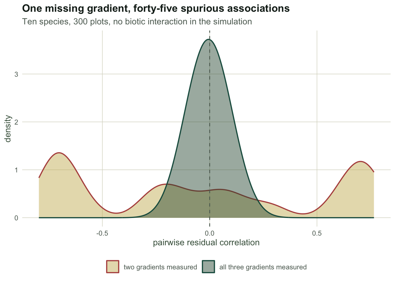
The algebra says the mechanisms cannot be told apart. The simulation below says something more practical: an ordinary unrecorded gradient, with no biotic interaction anywhere, is enough to fill the matrix with residual correlation, and its effect is large.
Ten species respond to three environmental gradients. Two are measured. The third is real, ordinary and unrecorded: soil depth, say, or grazing history. There is no interaction anywhere in the code.
set.seed(385)
n <- 300L
Sp <- 10L
x1 <- runif(n, -2, 2)
x2 <- runif(n, -2, 2)
x3 <- runif(n, -2, 2)

b1 <- rnorm(Sp, 0, 0.8)
b2 <- rnorm(Sp, 0, 0.6)
b3 <- c(1.2, 1.1, 0.9, 0.8, 0.7, -0.9, -1.0, -1.1, 0.1, -0.2)
a0 <- rnorm(Sp, 2, 0.5)

Y <- outer(rep(1, n), a0) + outer(x1, b1) + outer(x2, b2) + outer(x3, b3) +
     matrix(rnorm(n * Sp, 0, 0.7), n, Sp)

lower <- lower.tri(diag(Sp))
R_short <- cor(residuals(lm(Y ~ x1 + x2)))
R_full  <- cor(residuals(lm(Y ~ x1 + x2 + x3)))

## k is the number of variables partialled out, so the z has sqrt(n - 3 - k)
z_test <- function(r, nn, k) 2 * pnorm(-abs(atanh(r) * sqrt(nn - 3 - k)))
flag_short <- sum(z_test(R_short[lower], n, 2) < 0.05)
flag_full  <- sum(z_test(R_full[lower], n, 3) < 0.05)
npairs <- sum(lower)
Fitting the two measured gradients leaves an average absolute residual correlation of 0.494, with the strongest pair at 0.796. Tested pair by pair at the five per cent level, 39 of the 45 pairs come out significant. Add the third gradient and the average falls to 0.055, the strongest pair to 0.140, and the count of significant pairs to 4.
A proxy is not a substitute
The obvious response is that nobody measures everything, so use whatever you have. The question is how good a stand-in has to be before it helps.
set.seed(3851)
rhos <- c(0, 0.3, 0.6, 0.9, 0.99)
z3 <- as.numeric(scale(x3))  # x3 is not unit-variance, so standardise it first
proxy_mean <- sapply(rhos, function(rho) {
  e <- residuals(lm(rnorm(n) ~ z3)); e <- e / sd(e)  # unit-variance noise uncorrelated with z3
  prox <- rho * z3 + sqrt(1 - rho^2) * e             # so cor(prox, x3) is exactly rho
  Rp <- cor(residuals(lm(Y ~ x1 + x2 + prox)))
  mean(abs(Rp[lower]))
})
base_mean <- mean(abs(R_short[lower]))
removed <- 1 - proxy_mean / base_mean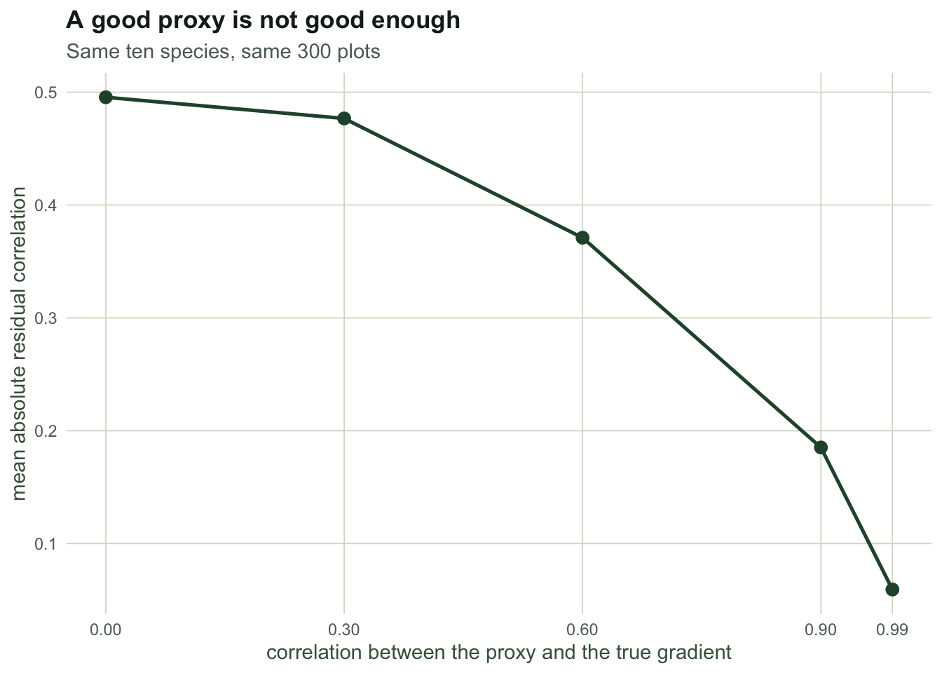
A proxy correlating 0.6 with the truth, which would count as a strong covariate in most surveys, removes only 16 per cent of the spurious structure. At 0.9 it removes 56 per cent. The relationship is steeply nonlinear because what survives is the component of the gradient the proxy misses, and that component still drives every species.
What survives
The residual correlation matrix does carry information, and it is worth being precise about what kind.
It is evidence that the fitted environmental model is incomplete. That is a real and useful finding: a strongly structured residual correlation matrix says your covariates are not enough, in the same way a patterned residual plot does in an ordinary regression.
It is a good basis for prediction, as the first post in this series measured. Conditional prediction does not require knowing why species covary, only that they do.
It is not evidence of interaction, and adding species traits, phylogeny or spatial random effects does not change that. Those additions can explain the correlation better; none of them can rule out an unrecorded gradient, because the unrecorded gradient produces exactly the same distribution.
The honest reporting standard follows from that. Call the entries associations, not interactions. State what environment was measured and what was not. If the question really is whether species A suppresses species B, the answer comes from a removal experiment or a designed gradient, not from a bigger observational matrix.
References
Blanchet, Cazelles, Gravel 2020 Ecology Letters 23(7):1050-1063 (10.1111/ele.13525)
Dormann, Bobrowski, Dehling, Harris, Hartig, Lischke, Moretti, Pagel, Pinkert, Schleuning, Schmidt, Sheppard, Steinbauer, Zeuss, Kraan 2018 Global Ecology and Biogeography 27(9):1004-1016 (10.1111/geb.12759)
Poggiato, Munkemuller, Bystrova, Arbel, Clark, Thuiller 2021 Trends in Ecology and Evolution 36(5):391-401 (10.1016/j.tree.2021.01.002)
Zurell, Pollock, Thuiller 2018 Ecography 41(11):1812-1819 (10.1111/ecog.03315)