library(ggplot2)

theme_te <- function(base_size = 11) {
  theme_minimal(base_size = base_size) +
    theme(panel.grid.minor = element_blank(),
          panel.grid.major = element_line(colour = "#dad9ca", linewidth = 0.3),
          axis.title = element_text(colour = "#46604a"),
          axis.text = element_text(colour = "#5d6b61"),
          plot.title = element_text(colour = "#16241d", face = "bold"),
          plot.subtitle = element_text(colour = "#5d6b61"),
          legend.title = element_text(colour = "#46604a"),
          legend.text = element_text(colour = "#5d6b61"),
          strip.text = element_text(colour = "#16241d"),
          plot.background = element_rect(fill = "#f5f4ee", colour = NA),
          panel.background = element_rect(fill = "#f5f4ee", colour = NA))
}

set.seed(383)

n <- 200L
S <- 12L
moisture <- runif(n, -2, 2)
openness <- runif(n, -2, 2)
X <- cbind(1, moisture, openness)
p <- ncol(X)

B_true <- cbind(rnorm(S, 2.0, 0.6), rnorm(S, 0.0, 0.9), rnorm(S, 0.0, 0.7))

Lam <- cbind(c( 0.9,  0.8,  0.7,  0.6, -0.7, -0.8, -0.6,  0.1, 0.0, 0.2, -0.1,  0.3),
             c( 0.2, -0.1,  0.3,  0.5,  0.4, -0.2,  0.6, -0.8, -0.7, 0.7,  0.8, -0.6))
psi_true <- rep(0.35, S)
Sigma_true <- Lam %*% t(Lam) + diag(psi_true)
R_true <- cov2cor(Sigma_true)

Y <- X %*% t(B_true) + matrix(rnorm(n * S), n, S) %*% chol(Sigma_true)
colnames(Y) <- paste0("sp", sprintf("%02d", seq_len(S)))Joint species distribution models in R
R
JSDM
community ecology
ecology tutorial
ggplot2
Fit a whole community at once in R: what joint modelling changes, what it leaves exactly unchanged, and why the residual correlation matrix is the real product.
Corrected 14 October 2026: the section on uneven sampling called the variance gain for the weakly correlated species nothing and said that the joint model borrows information only where the designs differ; it now calls that gain almost nothing and limits the second claim to Gaussian responses.
Corrected 7 October 2026: the post said that a shared design was all it took for joint fitting to leave every environmental coefficient unchanged; it now limits that to Gaussian responses, as the takeaway already did, and it calls the variation left after the measured environment not just noise, since part of it is independent noise.
Corrected 30 September 2026: the takeaway said joint fitting never changes species-environment coefficients on balanced data; it now limits that to Gaussian responses, since for presence-absence and count models the cancellation is not exact.
You surveyed 200 plots and recorded the cover of twelve fen plants. The obvious analysis is twelve regressions: cover against soil moisture and canopy openness, one species at a time. Every species gets its own slopes, and the community is whatever you get when you stack the twelve outputs next to each other.
A joint species distribution model refuses to stack. It writes down one model for the whole matrix of responses, with a covariance between species built into it. The promise is appealing: species that turn up together more often than the environment explains will show up as a positive residual correlation, and you can read the community off that matrix.
Before reaching for a package it is worth knowing exactly which part of that promise is real. This post sets up the model on the easy case, a Gaussian response on the log scale, and measures three things: what the joint fit changes, what it leaves untouched, and what it buys you that the stacked fit cannot.
A synthetic fen
Twelve species, 200 plots, two measured gradients. The residual covariance is built from two hidden gradients that the survey never recorded, so species share structure beyond moisture and openness.
The environment does real work here. Across the twelve species the median proportion of variance explained by moisture and openness alone is
r2_env <- sapply(seq_len(S), function(j) summary(lm(Y[, j] ~ moisture + openness))$r.squared)
r2_med <- median(r2_env)
0.719, with a range of 0.229 to 0.893. What is left over is not just noise: it carries the two hidden gradients.
One species at a time, then all at once
The stacked analysis is twelve calls to lm. The joint analysis treats the whole response matrix as multivariate normal with covariance Sigma across species, and estimates the coefficients by generalised least squares. Both are written out below, the second using the true Sigma so that nothing is hidden behind an estimation step.
B_stacked <- t(sapply(seq_len(S), function(j) coef(lm(Y[, j] ~ moisture + openness))))

Sinv <- solve(Sigma_true)
A <- kronecker(Sinv, crossprod(X))
b <- as.vector(crossprod(X, Y) %*% Sinv)
B_joint <- t(matrix(solve(A, b), p, S))

sur_gap <- max(abs(B_joint - B_stacked))
Every joint coefficient equals its stacked counterpart to within floating-point rounding, and that is not a coincidence of this data set. When every species is regressed on the same design matrix, the generalised least squares estimator collapses algebraically to equation-by-equation ordinary least squares. The covariance between species cancels out of the estimating equations entirely. This is the seemingly unrelated regressions result from econometrics, and it holds exactly.
So the first honest statement about joint modelling is a negative one. If all your species were measured at the same plots with the same predictors and the responses are Gaussian, fitting them jointly will not move a single environmental coefficient.
What the joint model actually produces
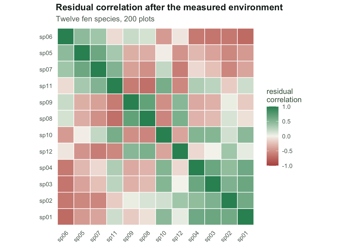
The product is the residual covariance. Because the coefficients are identical, the residuals are identical too, and their correlation can be read straight off the stacked fit.
Res <- Y - X %*% t(B_stacked)
R_hat <- cor(Res)
lower <- lower.tri(R_hat)

cor_recovery <- cor(R_hat[lower], R_true[lower])
max_gap <- max(abs(R_hat[lower] - R_true[lower]))
mean_abs <- mean(abs(R_hat[lower]))
strongest <- max(abs(R_hat[lower]))
Across the 66 species pairs the estimated residual correlations track the truth closely: the correlation between estimated and true values is 0.992, and no pair is off by more than 0.173. The average absolute residual correlation is 0.392 and the strongest pair reaches 0.722.
The thing the stacked model cannot do
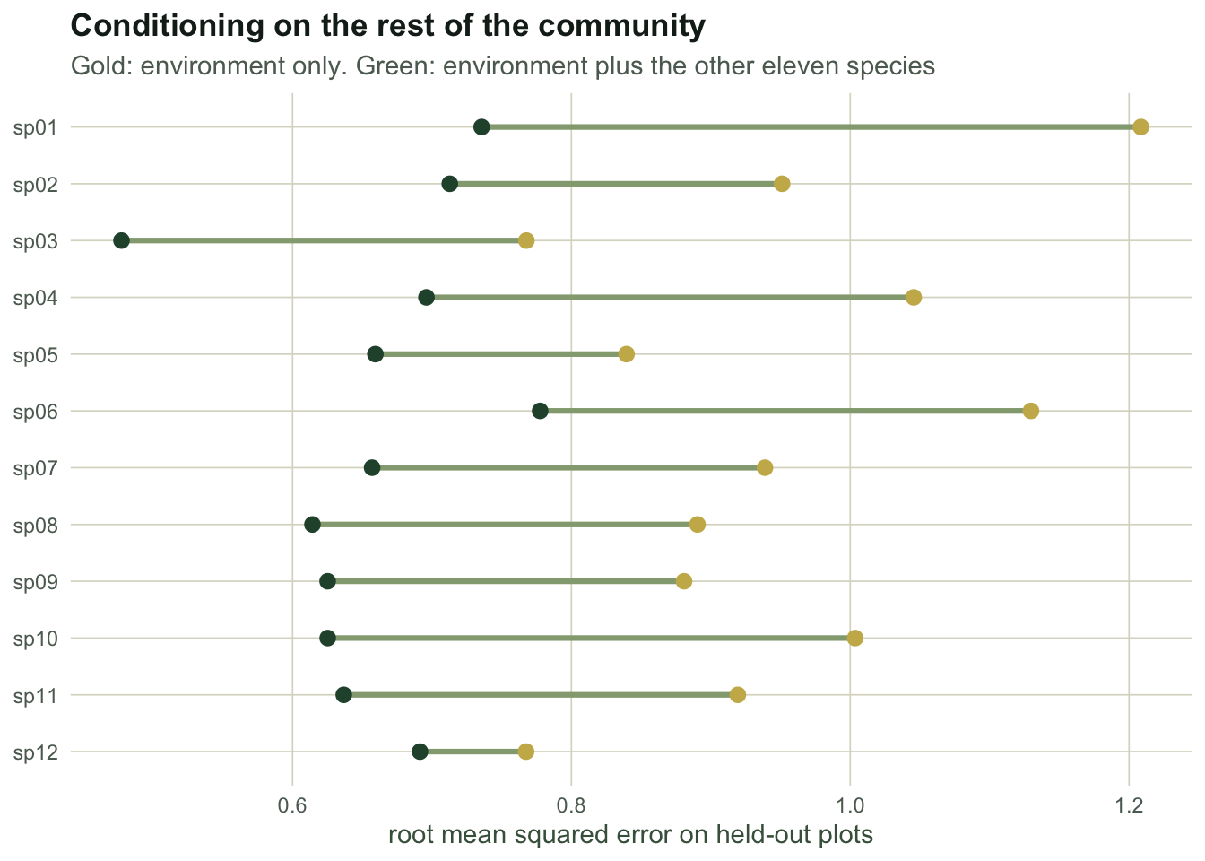
Here is where the joint model earns its keep. Suppose you visit a new plot, measure moisture and openness, and want a prediction for one species. The stacked model gives you the marginal expectation and stops. But at a real plot you often know more than the environment: you have already recorded the other eleven species. The joint model turns that into a conditional prediction, because the residual covariance tells you how to update species j once the other residuals are observed.
set.seed(3831)
holdout <- sample(n, 60)
train <- setdiff(seq_len(n), holdout)

B_tr <- t(sapply(seq_len(S), function(j)
  coef(lm(Y[train, j] ~ moisture[train] + openness[train]))))
Res_tr <- Y[train, ] - X[train, ] %*% t(B_tr)
S_tr <- cov(Res_tr)

Mu <- X[holdout, ] %*% t(B_tr)
pred_cond <- Mu
for (j in seq_len(S)) {
  w <- S_tr[j, -j, drop = FALSE] %*% solve(S_tr[-j, -j])
  pred_cond[, j] <- Mu[, j] + as.vector((Y[holdout, -j] - Mu[, -j]) %*% t(w))
}

rmse <- function(a, b) sqrt(mean((a - b)^2))
rmse_marg <- rmse(Mu, Y[holdout, ])
rmse_cond <- rmse(pred_cond, Y[holdout, ])
gain <- 1 - rmse_cond / rmse_marg

per_species <- sapply(seq_len(S), function(j)
  1 - rmse(pred_cond[, j], Y[holdout, j]) / rmse(Mu[, j], Y[holdout, j]))
On 60 held-out plots the environment-only prediction has a root mean squared error of 0.954. Conditioning on the other species drops it to 0.663, a reduction of 30.5 per cent. The gain is not shared equally: the best-served species improves by 39.1 per cent and the worst by 9.9 per cent.
When joint fitting does move the coefficients
For Gaussian responses, the exact cancellation above needed one thing: a common design matrix. Break that and the joint model starts doing real estimation work. The common way to break it in ecology is uneven sampling. A hard-to-identify bryophyte gets recorded on a subset of plots; a species added to the protocol partway through has three seasons instead of eight.
The simulation below has four species, one of them recorded at only 50 of the 200 plots. Two of the four are strongly correlated in their residuals; the other two are nearly independent. The generalised least squares fit works plot by plot, using whichever species were observed there.
set.seed(3832)
n2 <- 200L
S2 <- 4L
Sig2 <- matrix(c(1.0, 0.8, 0.2, 0.0,
                 0.8, 1.0, 0.2, 0.0,
                 0.2, 0.2, 1.0, 0.1,
                 0.0, 0.0, 0.1, 1.0), S2, S2)
B2 <- rbind(c(2, 1.0), c(2, -0.5), c(2, 0.7), c(2, 0.3))

gls_missing <- function(Yc, Xm, Sig, obs) {
  q <- 2L
  A <- matrix(0, S2 * q, S2 * q)
  b <- numeric(S2 * q)
  for (i in seq_len(nrow(Xm))) {
    o <- which(obs[i, ])
    if (!length(o)) next
    V <- solve(Sig[o, o, drop = FALSE])
    Z <- matrix(0, length(o), S2 * q)
    for (k in seq_along(o)) Z[k, ((o[k] - 1) * q + 1):(o[k] * q)] <- Xm[i, ]
    A <- A + crossprod(Z, V) %*% Z
    b <- b + crossprod(Z, V) %*% Yc[i, o]
  }
  t(matrix(solve(A, b), q, S2))
}

run_gap <- function(target, reps) {
  keep <- matrix(NA_real_, reps, 2)
  for (r in seq_len(reps)) {
    xx <- runif(n2, -2, 2)
    Xm <- cbind(1, xx)
    Yf <- Xm %*% t(B2) + matrix(rnorm(n2 * S2), n2, S2) %*% chol(Sig2)
    obs <- matrix(TRUE, n2, S2)
    obs[sample(n2, 150), target] <- FALSE
    Yc <- Yf
    Yc[!obs] <- NA
    keep[r, ] <- c(coef(lm(Yc[, target] ~ xx))[2],
                   gls_missing(Yc, Xm, Sig2, obs)[target, 2])
  }
  keep
}

k_linked <- run_gap(1L, 400L)
k_alone  <- run_gap(3L, 200L)

sd_st <- sd(k_linked[, 1]); sd_jt <- sd(k_linked[, 2])
vr_linked <- var(k_linked[, 1]) / var(k_linked[, 2])
vr_alone  <- var(k_alone[, 1]) / var(k_alone[, 2])
For the sparsely recorded species that correlates 0.8 with a fully recorded neighbour, the stacked slope has a standard deviation of 0.1255 across replicates and the joint slope 0.0910: a variance ratio of 1.90 in favour of the joint fit, with both estimators unbiased (stacked bias -0.0027, joint bias +0.0042).
Run the same experiment on the species whose strongest residual correlation with anything else is 0.2, and the ratio falls to 1.05. That is almost nothing. The gain comes from the correlation, not from the jointness: the joint model borrows information across species only to the extent that the species are actually correlated, and, for Gaussian responses, only where the designs differ.
What to take away
Three measured statements, in order of how often they get muddled.
For Gaussian responses, joint fitting does not change species-environment coefficients on balanced data. The exact cancellation is worth remembering the next time a reviewer asks why you did not fit a joint model to such data: if the design is common, it would give the same numbers. For presence-absence or count responses the cancellation is not exact, and the coefficients can move.
The residual correlation matrix is the actual output, and you can compute it from stacked residuals for Gaussian responses. Its value is that it becomes an estimable object with a structure and an uncertainty, which matters more for presence-absence and count data where the residuals are not directly available.
Conditional prediction is the concrete gain. If you will ever predict one species at a site where others have been recorded, the joint model is the tool that uses that information.
What the matrix does not tell you is where the structure came from. In this simulation it came from two hidden environmental gradients and no biotic interaction whatsoever, and nothing in the fitted correlations distinguishes that from competition. That is the subject of a later post in this series.
References
Ovaskainen, Tikhonov, Norberg, Blanchet, Duan, Dunson, Roslin, Abrego 2017 Ecology Letters 20(5):561-576 (10.1111/ele.12757)
Pollock, Tingley, Morris, Golding, O’Hara, Parris, Vesk, McCarthy 2014 Methods in Ecology and Evolution 5(5):397-406 (10.1111/2041-210X.12180)
Warton, Blanchet, O’Hara, Ovaskainen, Taskinen, Walker, Hui 2015 Trends in Ecology and Evolution 30(12):766-779 (10.1016/j.tree.2015.09.007)