library(ggplot2)

theme_te <- function(base_size = 11) {
  theme_minimal(base_size = base_size) +
    theme(panel.grid.minor = element_blank(),
          panel.grid.major = element_line(colour = "#dad9ca", linewidth = 0.3),
          axis.title = element_text(colour = "#46604a"),
          axis.text = element_text(colour = "#5d6b61"),
          plot.title = element_text(colour = "#16241d", face = "bold"),
          plot.subtitle = element_text(colour = "#5d6b61"),
          legend.title = element_text(colour = "#46604a"),
          legend.text = element_text(colour = "#5d6b61"),
          plot.background = element_rect(fill = "#f5f4ee", colour = NA),
          panel.background = element_rect(fill = "#f5f4ee", colour = NA))
}

set.seed(384)

n <- 200L
S <- 12L
Lam0 <- cbind(c( 0.9,  0.8,  0.7,  0.6, -0.7, -0.8, -0.6,  0.1, 0.0, 0.2, -0.1,  0.3),
              c( 0.2, -0.1,  0.3,  0.5,  0.4, -0.2,  0.6, -0.8, -0.7, 0.7,  0.8, -0.6))
psi0 <- rep(0.35, S)
Sigma0 <- Lam0 %*% t(Lam0) + diag(psi0)
R0 <- cov2cor(Sigma0)

moisture <- runif(n, -2, 2)
openness <- runif(n, -2, 2)
B <- cbind(rnorm(S, 2, 0.6), rnorm(S, 0, 0.9), rnorm(S, 0, 0.7))
Y <- cbind(1, moisture, openness) %*% t(B) +
     matrix(rnorm(n * S), n, S) %*% chol(Sigma0)
colnames(Y) <- paste0("sp", sprintf("%02d", seq_len(S)))

Res <- residuals(lm(Y ~ moisture + openness))
C_sample <- cov(Res)
R_sample <- cor(Res)
lower <- lower.tri(R0)Latent variables and species correlations
R
JSDM
community ecology
ecology tutorial
ggplot2
Shrink a species correlation matrix with latent factors in R: the exact rotation invariance, how to choose the number of factors, and what low rank really buys.
Corrected 1 October 2026: the comparison of the number of factors used EM fits that, above two factors, had stopped short of the maximum likelihood fit, some of them at a local optimum; it now fits every number of factors with factanal from many starting points, which moves two quoted distances in their last decimal place and changes no conclusion.
Corrected 27 September 2026: the post said all three criteria for the number of factors agree with the true two; only the likelihood ratio test and the held-out likelihood do, while the in-sample fit keeps improving with more factors.
A joint model for S species carries a residual covariance matrix with S(S+1)/2 free entries. Twelve species is 78 numbers. Fifty species is 1275, which is more parameters than most surveys have plots. Somewhere between those two the unstructured matrix stops being an estimate and starts being a rearrangement of the data.
The standard fix is to assume the residual structure is low dimensional: a handful of unmeasured gradients that all species respond to, plus species-specific noise. That is a factor model, and in the ecological literature it arrives under the name latent variable joint species distribution model. This post builds it by hand, measures the one property that most trips people up, and tests three ways of choosing how many factors to use.
The model
Write the residual covariance as a low-rank part plus a diagonal. With k latent gradients, each species gets k loadings and one uniqueness, which brings 78 numbers down to 36 for two factors, and 1275 down to 150 for fifty species.
The loadings are not identified, and this is exact
Before fitting anything, one property deserves to be measured rather than asserted. Take any orthogonal rotation of the loading matrix. The implied covariance does not change at all.
theta <- 0.7
Q <- matrix(c(cos(theta), -sin(theta), sin(theta), cos(theta)), 2, 2)
orth_gap <- max(abs(crossprod(Q) - diag(2)))

Lam_rot <- Lam0 %*% Q
rot_gap <- max(abs(Lam_rot %*% t(Lam_rot) - Lam0 %*% t(Lam0)))
The rotation matrix is orthogonal (its cross-product equals the identity to within floating-point rounding), and the rotated loadings reproduce the original covariance to within floating-point rounding as well. Meanwhile the individual loadings have moved a long way: species 1 loads 0.90 on the first factor before rotation and 0.56 after, and species 8 goes from 0.10 to 0.59.
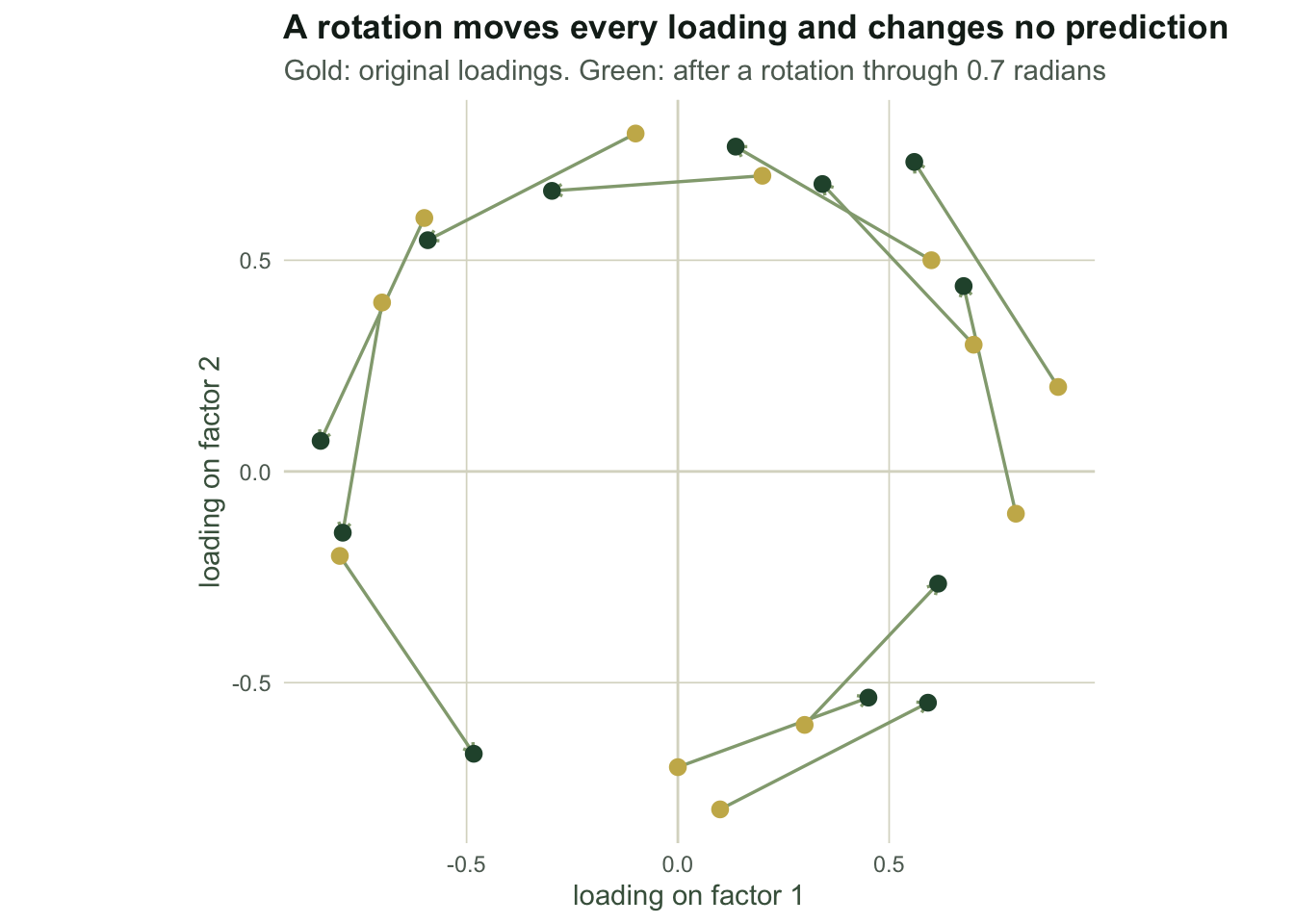
The practical consequence is blunt. A statement of the form “species 10 loads positively on the first latent axis, which we interpret as a moisture gradient” has no content on its own: the rotation above already turns that loading negative, and another angle sends it anywhere on the circle. What is identified is the matrix of implied correlations between species, and any summary computed from it. Ordination plots from latent variable models are legitimate as displays of relative position, which is exactly how model-based ordination treats them, but the axes themselves carry no privileged meaning.
Fitting the factor model
The expectation-maximisation algorithm for a factor model is short enough to write out. Each iteration computes the conditional moments of the latent scores given the current parameters, then updates the loadings and uniquenesses from those moments.
fa_em <- function(Cmat, k, iter = 2000, tol = 1e-10) {
  d <- sqrt(diag(Cmat))
  R <- Cmat / outer(d, d)
  ev <- eigen(R, symmetric = TRUE)
  Lam <- ev$vectors[, seq_len(k), drop = FALSE] %*%
         diag(sqrt(pmax(ev$values[seq_len(k)], 1e-6)), k)
  psi <- pmax(diag(R) - rowSums(Lam^2), 1e-3)
  ll_old <- -Inf
  for (it in seq_len(iter)) {
    Sinv <- solve(Lam %*% t(Lam) + diag(psi))
    beta <- t(Lam) %*% Sinv
    Ezz <- diag(k) - beta %*% Lam + beta %*% R %*% t(beta)
    Lam <- R %*% t(beta) %*% solve(Ezz)
    psi <- pmax(diag(R - Lam %*% beta %*% R), 1e-4)
    Sg <- Lam %*% t(Lam) + diag(psi)
    ll <- -0.5 * (determinant(Sg, logarithm = TRUE)$modulus[1] + sum(diag(solve(Sg, R))))
    if (abs(ll - ll_old) < tol) break
    ll_old <- ll
  }
  list(loadings = Lam, uniquenesses = psi,
       Sigma = Lam %*% t(Lam) + diag(psi), iter = it)
}

fit2 <- fa_em(C_sample, 2)
R_fit <- cov2cor(fit2$Sigma)

gap_fit <- max(abs(R_fit[lower] - R0[lower]))
rmse_fit <- sqrt(mean((R_fit[lower] - R0[lower])^2))
rmse_raw <- sqrt(mean((R_sample[lower] - R0[lower])^2))
It converges in 54 iterations. The fitted correlations sit within 0.071 of the truth, with a root mean squared error of 0.0351 against 0.0402 for the raw sample correlations.
As a private check the same model is available in base R through factanal, which uses a different optimiser and a different convergence rule.
fa_pkg <- factanal(covmat = R_sample, factors = 2, n.obs = n, rotation = "none")
L_pkg <- fa_pkg$loadings[, ]
R_pkg <- L_pkg %*% t(L_pkg) + diag(fa_pkg$uniquenesses)
pkg_gap <- max(abs(R_pkg - R_fit))
The two implied correlation matrices agree to \(6.0 \times 10^{-6}\). That is not machine precision and should not be: two optimisers stopping at different tolerances agree far more closely than any number quoted in this post, which is enough to say the hand-written version is correct.
How many factors
Three criteria, each answering a slightly different question. The first is the fit to the observed correlation matrix; the second is a likelihood ratio test; the third is the held-out likelihood.
Beyond two factors the hand-written EM slows to a crawl, stops at its iteration cap and can settle on a local optimum, so the comparison below fits every k with factanal() from many starting points instead. At one and two factors the two fitters agree.
fa_ml <- function(Cmat, k) {
  fp <- factanal(covmat = cov2cor(Cmat), factors = k, rotation = "none",
                 control = list(nstart = 30, lower = 1e-4))
  L <- fp$loadings[, , drop = FALSE]
  list(Sigma = L %*% t(L) + diag(fp$uniquenesses))
}

ks <- 1:6
tab <- t(sapply(ks, function(k) {
  f <- fa_ml(C_sample, k)
  Rk <- cov2cor(f$Sigma)
  c(to_sample = sqrt(mean((Rk[lower] - R_sample[lower])^2)),
    to_truth  = sqrt(mean((Rk[lower] - R0[lower])^2)))
}))
best_truth <- ks[which.min(tab[, "to_truth"])]

set.seed(3842)
ho <- sample(n, 70)
tr <- setdiff(seq_len(n), ho)
Res_tr <- residuals(lm(Y[tr, ] ~ moisture[tr] + openness[tr]))
Res_ho <- residuals(lm(Y[ho, ] ~ moisture[ho] + openness[ho]))
C_tr <- cov(Res_tr)
ll_out <- sapply(ks, function(k) {
  f <- fa_ml(C_tr, k)
  d <- sqrt(diag(C_tr))
  Sg <- f$Sigma * outer(d, d)
  -0.5 * (nrow(Res_ho) * determinant(Sg, logarithm = TRUE)$modulus[1] +
          sum(Res_ho %*% solve(Sg) * Res_ho))
})
best_ho <- ks[which.max(ll_out)]

lr <- t(sapply(1:3, function(k) {
  fk <- factanal(covmat = R_sample, factors = k, n.obs = n)
  c(stat = unname(fk$STATISTIC), df = unname(fk$dof), p = unname(fk$PVAL))
}))
The likelihood ratio test rejects one factor decisively (statistic 879.2 on 54 degrees of freedom, p below 0.0001) and does not reject two (statistic 51.8 on 43 degrees of freedom, p = 0.167). The held-out likelihood peaks at 2 factors, rising from -354 at one factor to -155 at two and falling steadily afterwards. Both agree with the simulation, which had two; the first criterion, the fit to the observed correlation matrix, does not.
The interesting part is the divergence between the two curves below.
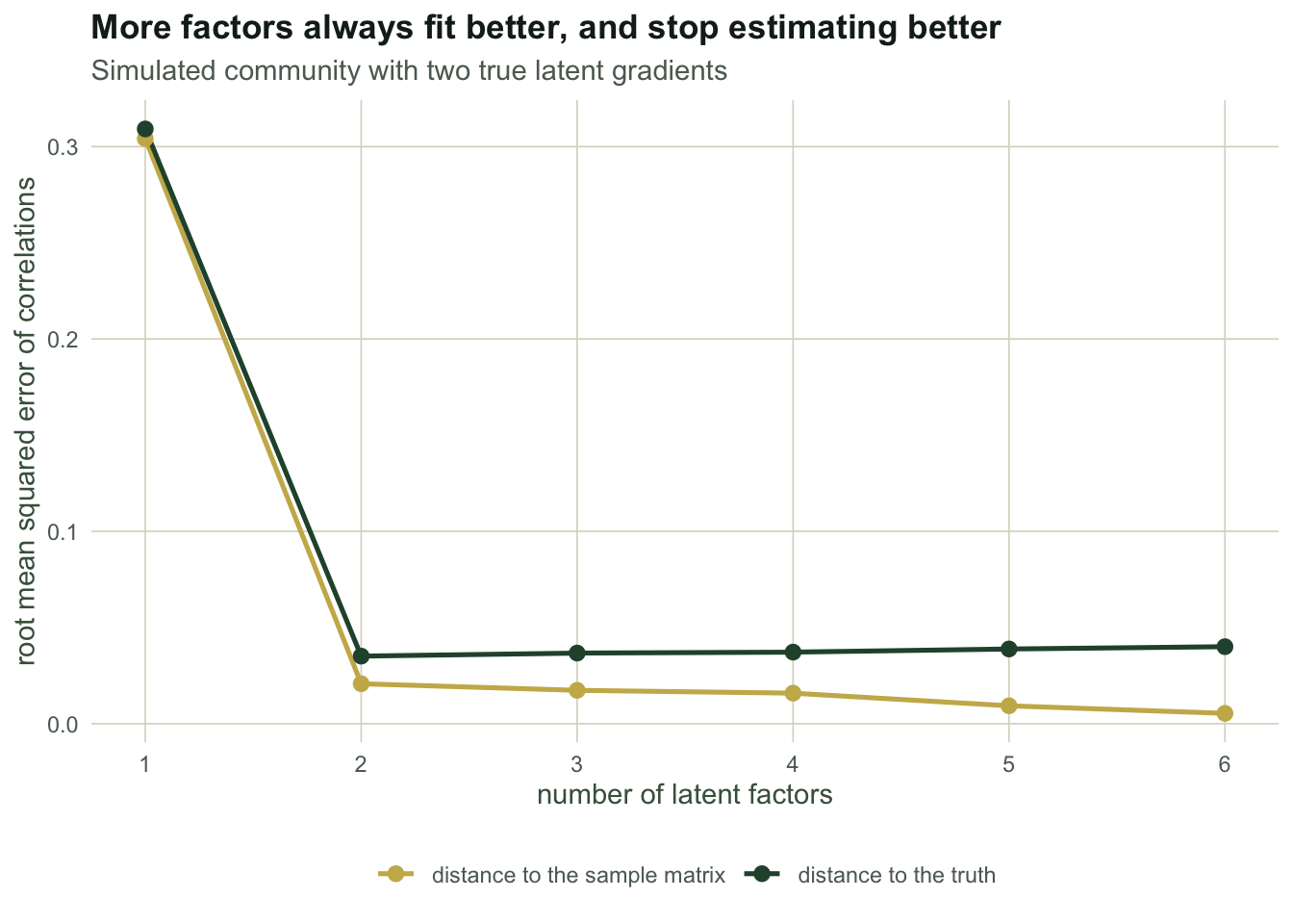
Going from two factors to six cuts the distance to the sample matrix from 0.0207 to 0.0052, while the distance to the truth grows from 0.0351 to 0.0401. This is the ordinary overfitting signature, and it is the reason the in-sample fit cannot be used to pick k. The minimum against the truth is at 2 factors, which you would never see with real data. The held-out likelihood is the closest usable stand-in.
What the low-rank model is actually for
There is a temptation to sell the factor model as a precision device. Measure it instead.
set.seed(3841)
sweep_n <- function(nn, reps = 40) {
  out <- matrix(NA_real_, reps, 2)
  for (r in seq_len(reps)) {
    m1 <- runif(nn, -2, 2)
    m2 <- runif(nn, -2, 2)
    Yn <- cbind(1, m1, m2) %*% t(B) + matrix(rnorm(nn * S), nn, S) %*% chol(Sigma0)
    Rn <- residuals(lm(Yn ~ m1 + m2))
    Rs <- cor(Rn)
    Rk <- cov2cor(fa_em(cov(Rn), 2)$Sigma)
    out[r, ] <- c(sqrt(mean((Rs[lower] - R0[lower])^2)),
                  sqrt(mean((Rk[lower] - R0[lower])^2)))
  }
  colMeans(out)
}
grid_n <- c(40, 60, 100, 200, 400)
sw <- t(sapply(grid_n, sweep_n))
ratio <- sw[, 1] / sw[, 2]

set.seed(3843)
rank_at <- function(nn) {
  m1 <- runif(nn, -2, 2); m2 <- runif(nn, -2, 2)
  Yn <- cbind(1, m1, m2) %*% t(B) + matrix(rnorm(nn * S), nn, S) %*% chol(Sigma0)
  qr(cor(residuals(lm(Yn ~ m1 + m2))))$rank
}
rk10 <- rank_at(10L)
rk14 <- rank_at(14L)
Across plot counts from 40 to 400, the two-factor estimate beats the raw sample correlation by a ratio of 1.07 to 1.08 in root mean squared error. That is a real improvement and a small one, and it does not grow as the sample shrinks.
The feasibility argument is much stronger than the precision argument. With 10 plots and twelve species the sample residual correlation matrix has rank 7; with 14 plots, rank 11. A singular matrix cannot be inverted, so the conditional prediction from the previous post is not merely imprecise, it is undefined. The factor model has no such failure: it fits 36 parameters regardless of how many plots you have, and returns a positive definite matrix every time.
So the honest summary is that latent factors buy you a model that exists, an ordination you can plot, and a parameter count that does not scale quadratically with the species list. They do not buy you much accuracy per pair, and they do not turn a small survey into a big one.
References
Hui 2016 Methods in Ecology and Evolution 7(6):744-750 (10.1111/2041-210X.12514)
Ovaskainen, Tikhonov, Norberg, Blanchet, Duan, Dunson, Roslin, Abrego 2017 Ecology Letters 20(5):561-576 (10.1111/ele.12757)
Warton, Blanchet, O’Hara, Ovaskainen, Taskinen, Walker, Hui 2015 Trends in Ecology and Evolution 30(12):766-779 (10.1016/j.tree.2015.09.007)