library(ggplot2)

theme_te <- function(base_size = 11) {
  theme_minimal(base_size = base_size) +
    theme(panel.grid.minor = element_blank(),
          panel.grid.major = element_line(colour = "#dad9ca", linewidth = 0.3),
          axis.title = element_text(colour = "#46604a"),
          axis.text = element_text(colour = "#5d6b61"),
          plot.title = element_text(colour = "#16241d", face = "bold"),
          plot.subtitle = element_text(colour = "#5d6b61"),
          legend.title = element_text(colour = "#46604a"),
          legend.text = element_text(colour = "#5d6b61"),
          plot.background = element_rect(fill = "#f5f4ee", colour = NA),
          panel.background = element_rect(fill = "#f5f4ee", colour = NA))
}

set.seed(386)

null_max <- function(S, n, B) {
  off <- lower.tri(diag(S))
  replicate(B, {
    Z <- matrix(rnorm(n * S), n, S)
    x <- runif(n, -2, 2)
    R <- cor(residuals(lm(Z ~ x)))
    max(abs(R[off]))
  })
}

n_plots <- 100L
S_grid <- c(5L, 10L, 20L, 40L)
null_tab <- t(sapply(S_grid, function(S) {
  m <- null_max(S, n_plots, 600L)
  c(pairs = S * (S - 1) / 2, med = median(m), hi = unname(quantile(m, 0.95)))
}))Checking a joint species distribution model
R
JSDM
community ecology
ecology tutorial
ggplot2
Three checks for a species association matrix in R: how big the strongest pair gets under a null, what presence-absence costs, and what missing effort does.
Corrected 30 September 2026: the post turned the squared ratio of standard deviations into the number of extra plots a presence-absence survey needs, which assumes the spread falls with the square root of the plot count; that does not hold at this plot count and prevalence, and the post now says the multiple is several times and smaller than the squared ratio suggests.
Suppose the identification problem from the previous post has been faced squarely: the matrix is being reported as associations, not interactions, and the discussion is careful. There are still three ways for a species association matrix to mislead that have nothing to do with mechanism and everything to do with sampling. All three are measurable before the results are written up.
Check one: how big is the strongest pair when nothing is going on
A matrix for S species contains S(S-1)/2 pairs. Every one is estimated with error, and the number people look at first is the largest. That makes it an extreme value, and extreme values grow with the number of draws.
The simulation below has no associations at all: independent species, one shared covariate, correlations computed from the residuals exactly as in a real analysis.
With 10 species (45 pairs) and 100 plots, the largest absolute residual correlation is 0.239 in a typical data set and reaches 0.323 in one survey out of twenty. At 40 species (780 pairs) those numbers rise to 0.331 and 0.392, and every single one of those associations is pure noise.
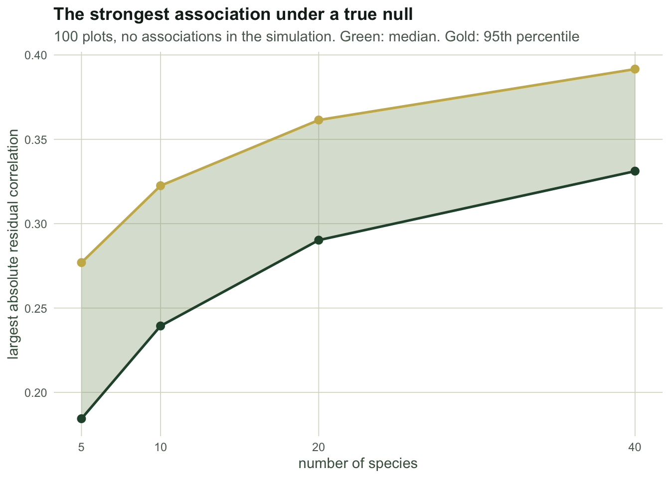
The check is cheap to run on your own design: simulate independent species at your plot count and richness, and record the distribution of the maximum. If your headline pair does not clear that distribution, it is not a finding. Note that this is the same multiplicity problem that false discovery rate methods were built for, with one twist: the pairs are not independent of each other, so a naive correction over S(S-1)/2 tests is not right either. The simulated null handles the dependence for free.
Check two: what presence-absence data cost
Most of the JSDM literature is written for presence-absence, and most of the reassuring simulations are run on abundance. The difference is large enough to change what a survey can support.
Thresholding a latent variable at a prevalence throws away most of the information about the correlation. The estimator that recovers it is the tetrachoric correlation: the correlation of the underlying normal pair implied by a two by two table of joint occurrences. It needs a bivariate normal probability, which can be written as a one-dimensional integral.
bvn <- function(h, k, rho) {
  s <- sqrt(1 - rho^2)
  integrate(function(z) pnorm((k - rho * z) / s) * dnorm(z),
            lower = -8, upper = h, rel.tol = 1e-8)$value
}

tetrachoric <- function(y1, y2) {
  h <- qnorm(mean(y1 == 0)); k <- qnorm(mean(y2 == 0))
  if (!is.finite(h) || !is.finite(k)) return(NA_real_)
  cnt <- c(sum(y1 == 0 & y2 == 0), sum(y1 == 0 & y2 == 1),
           sum(y1 == 1 & y2 == 0), sum(y1 == 1 & y2 == 1))
  nll <- function(rho) {
    p00 <- bvn(h, k, rho)
    p <- pmax(c(p00, pnorm(h) - p00, pnorm(k) - p00,
                1 - pnorm(h) - pnorm(k) + p00), 1e-12)
    -sum(cnt * log(p))
  }
  optimize(nll, c(-0.95, 0.95), tol = 1e-4)$minimum
}

rho_true <- 0.6
compare <- function(nn, prevalence, B) {
  cutoff <- qnorm(1 - prevalence)
  Ch <- chol(matrix(c(1, rho_true, rho_true, 1), 2, 2))
  g <- numeric(B); b <- numeric(B)
  for (i in seq_len(B)) {
    Z <- matrix(rnorm(2 * nn), nn, 2) %*% Ch
    g[i] <- cor(Z[, 1], Z[, 2])
    b[i] <- tetrachoric(as.integer(Z[, 1] > cutoff), as.integer(Z[, 2] > cutoff))
  }
  c(sd_abund = sd(g), sd_pa = sd(b, na.rm = TRUE),
    bias_pa = mean(b, na.rm = TRUE) - rho_true)
}

set.seed(3861)
prev_grid <- c(0.50, 0.25, 0.10)
pa_tab <- t(sapply(prev_grid, function(p) compare(100L, p, 300L)))
ratio_pa <- pa_tab[, "sd_pa"] / pa_tab[, "sd_abund"]
At 100 plots and a true residual correlation of 0.6, the abundance-based estimate has a standard deviation of 0.062 to 0.067 across replicates, depending on the run. Reduced to presence-absence at a prevalence of 0.50, the standard deviation rises to 0.113, a factor of 1.8. At a prevalence of 0.10, which describes a great many real species, it rises to 0.347, a factor of 5.2 over the abundance run at that same prevalence, and the estimate also becomes biased towards zero by 0.061.
The practical translation: a presence-absence survey of rare species needs several times as many plots as an abundance survey to pin an association down equally well. That is usually not on offer, which is why so many published association matrices have credible intervals spanning zero for most pairs. Squaring the ratio above would put the multiple at 27, but that assumes the spread falls with the square root of the plot count, and at 100 plots and this prevalence the tetrachoric estimate is too skewed and bounded for that: its spread falls faster at first as plots are added, so the real multiple is smaller. To size a survey, rerun the comparison at the plot counts you are considering.
Check three: what unrecorded effort does
The third failure mode is the one most likely to be sitting in your own data. If plots differ in survey effort, area or observer skill, and that variation is not in the model, every species is inflated at the same plots. The result is a residual correlation matrix that is positive nearly everywhere.
set.seed(3862)
n2 <- 250L
Sp <- 10L
effort <- runif(n2, 0.5, 2)
env <- runif(n2, -2, 2)
slopes <- rnorm(Sp, 0, 0.8)
inter <- rnorm(Sp, 2, 0.4)

Yc <- outer(rep(1, n2), inter) + outer(env, slopes) +
      outer(log(effort), rep(1, Sp)) +
      matrix(rnorm(n2 * Sp, 0, 0.6), n2, Sp)

lower <- lower.tri(diag(Sp))
R_naive <- cor(residuals(lm(Yc ~ env)))
R_eff   <- cor(residuals(lm(Yc ~ env + log(effort))))
np <- sum(lower)
neg_naive <- sum(R_naive[lower] < 0)
neg_eff   <- sum(R_eff[lower] < 0)
Effort varies fourfold across plots and no species interacts with any other. Leaving effort out of the model gives a mean pairwise residual correlation of 0.247, and 0 of the 45 pairs come out negative. Putting effort in gives a mean of 0.003 with 18 of the 45 pairs negative: a matrix that straddles zero instead of sitting entirely on one side of it.
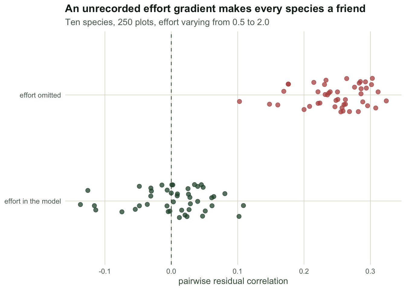
The diagnostic is simple and worth running on every fitted matrix: look at the sign balance. A community in which almost every pair is positively associated is far more likely to be telling you about sampling than about facilitation. The same signature comes from an unrecorded productivity gradient, from plots of unequal area, and from detection probability that varies by site.
Putting the three together
Each check answers a different question, and none of them is optional.
The null simulation says how large an association has to be before it is worth discussing at all, given your richness and plot count. The presence-absence comparison says whether your data type can support the question you are asking, which for rare species is often no. The sign balance says whether a shared sampling artefact is driving the whole matrix.
All three constrain rather than confirm, which is the pattern every checking post on this blog ends on. A matrix that survives them is still a matrix of associations of unknown cause. What the checks buy you is the removal of three specific ways of being wrong that have nothing to do with ecology.
References
Blanchet, Cazelles, Gravel 2020 Ecology Letters 23(7):1050-1063 (10.1111/ele.13525)
Dormann, Bobrowski, Dehling, Harris, Hartig, Lischke, Moretti, Pagel, Pinkert, Schleuning, Schmidt, Sheppard, Steinbauer, Zeuss, Kraan 2018 Global Ecology and Biogeography 27(9):1004-1016 (10.1111/geb.12759)
Pollock, Tingley, Morris, Golding, O’Hara, Parris, Vesk, McCarthy 2014 Methods in Ecology and Evolution 5(5):397-406 (10.1111/2041-210X.12180)
Zurell, Pollock, Thuiller 2018 Ecography 41(11):1812-1819 (10.1111/ecog.03315)