library(ggplot2)

te_pal <- list(forest = "#275139", green = "#2f8f63", sage = "#93a87f",
               clay = "#b5534e", gold = "#cda23f", line = "#dad9ca",
               ink = "#16241d", paper = "#f5f4ee")

theme_te <- function() {
  theme_minimal(base_size = 12) +
    theme(panel.grid.minor = element_blank(),
          panel.grid.major = element_line(colour = "#e7e6dc"),
          plot.background = element_rect(fill = "#f5f4ee", colour = NA),
          panel.background = element_rect(fill = "#f5f4ee", colour = NA),
          plot.title = element_text(face = "bold", colour = te_pal$ink),
          axis.title = element_text(colour = "#2c3a31"),
          axis.text = element_text(colour = "#2c3a31"),
          legend.position = "bottom")
}Copulas for dependent ecological data
R
multivariate
simulation
ecology tutorial
Separating dependence from marginals in R: why skewed ecological data cannot reach a target correlation, Sklar’s theorem by hand, and three copulas at one tau.
Two cliff-nesting seabird species have been counted at the same two colonies for thirty years, which gives sixty paired colony-years of an annual recruitment index for each species. The first species is steady: good years and bad years differ by a factor of two or three. The second collapses. In most years it produces a normal cohort, and every so often the whole colony fails and the index is close to zero.
A viability model now needs simulated futures for both species together, because the conservation question is about the probability that both populations are in trouble at the same time. The specification looks reasonable. Fit a lognormal to each species’ index, take the Pearson correlation between the two thirty-year series, and generate correlated pairs by the usual recipe: draw standard normals, multiply by the Cholesky factor of the target correlation matrix, and push each column through the fitted marginal quantile function.
The generated data comes back with a correlation well below the target. Raising the correlation in the Cholesky factor does not fix it. Setting the factor to its maximum, so that both columns are driven by the same standard normal, still does not fix it. Nothing is broken. The target was not attainable, and the reason has nothing to do with the sampler.
Correlation is a property of a joint distribution and not a free-standing quantity. Once you have chosen two marginal distributions you have already constrained the set of Pearson correlations that any joint distribution with those marginals can have, and for skewed ecological quantities that constraint bites hard. A copula is the object that separates the two questions: it holds the dependence structure with the marginals stripped out, so that the shape of the dependence and the shape of each variable can be chosen independently, up to the limits that this post measures.
That is not what the blog has done so far. Joint species distribution models in R and Latent variables and species correlations both build a residual covariance matrix and simulate with matrix(rnorm(n * S), n, S) %*% chol(Sigma), and so do a dozen other posts here. That single line is a Gaussian copula welded to normal marginals. It is a fine default and it is fast, but it can only produce one dependence shape, and when the marginals stop being normal it silently changes what the correlation coefficient means. Anderson et al (2019) set out the copula alternative for community data, in which each species keeps whatever marginal it has and the dependence between species is carried separately. The extreme-value cluster, Block maxima and the GEV distribution and its neighbours, is the other side of the gap: those posts model tails carefully but one variable at a time.
Four measurements follow. What the marginals allow a Pearson correlation to be; Sklar’s theorem run in both directions on one simulated dataset; three copulas calibrated to the same Kendall’s tau and what happens to the probability that both species fail in the same year; and whether a fitted comparison can tell those three apart at ecological sample sizes. No copula package is used. The bivariate Gaussian, Clayton and Gumbel copulas have short closed forms for the distribution function, the density and the sampler, and writing them out is the point.
What the marginals will let a correlation be
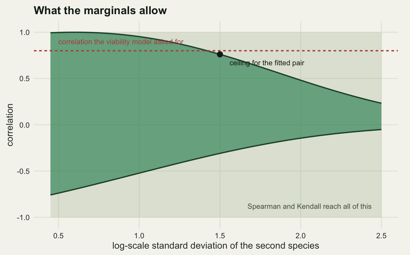
Take the two species as lognormal on the index scale, with log-scale standard deviations sig_a for the steady species and sig_b for the one that fails. The attainable range of Pearson correlation between two lognormals has a closed form, which makes it the cleanest possible demonstration. If both variables are driven by the same standard normal, the correlation is at its maximum; if one is driven by the negative of the other’s normal, it is at its minimum.
sig_a <- 0.6
sig_b <- 1.5
n_yr <- 30
n_pair <- 60
target_r <- 0.8

ln_bounds <- function(s1, s2) {
  den <- sqrt((exp(s1^2) - 1) * (exp(s2^2) - 1))
  c(lo = (exp(-s1 * s2) - 1) / den, hi = (exp(s1 * s2) - 1) / den)
}

cv_a <- sqrt(exp(sig_a^2) - 1)
cv_b <- sqrt(exp(sig_b^2) - 1)
bnd_here <- ln_bounds(sig_a, sig_b)
sig_seq <- c(0.6, 0.9, 1.2, 1.5, 1.8, 2.4)
bnd_tab <- cbind(sigma_b = sig_seq,
                 t(sapply(sig_seq, function(s) ln_bounds(sig_a, s))))
print(round(c(cv_steady = cv_a, cv_failing = cv_b), 4))
cv_steady cv_failing
0.6583 2.9134 print(round(bnd_tab, 4)) sigma_b lo hi
[1,] 0.6 -0.6977 1.0000
[2,] 0.9 -0.5674 0.9737
[3,] 1.2 -0.4345 0.8926
[4,] 1.5 -0.3094 0.7611
[5,] 1.8 -0.2025 0.5964
[6,] 2.4 -0.0652 0.2751The two fitted marginals have coefficients of variation of 0.6583 and 2.9134, which is what “steady” and “collapses” mean numerically. With those two marginals fixed, the Pearson correlation between the two species can be no larger than 0.7611 and no smaller than -0.3094. The specification asked for 0.8. There is no joint distribution with those marginals that has it, so no sampler can produce one, and the failure is not a numerical accident that a better algorithm would avoid.
The table shows how fast the ceiling drops. At a log-scale standard deviation of 0.9 for the second species the ceiling is still 0.9737; by 2.4 it is 0.2751, so two variables that both vary enormously and are perfectly monotonically related report a Pearson correlation a reader would describe as weak. The lower bound moves too, though not as far: at 2.4 the most negative correlation available is -0.0652. The attainable interval is not symmetric and it does not contain most of what a correlation coefficient is normally taken to span.
These are the Frechet-Hoeffding bounds, evaluated for a particular pair of marginals. The general statement is that any joint distribution function sits between two explicit envelopes built from the marginals alone, and those envelopes are themselves joint distributions: the upper one is the comonotone coupling, where both variables are increasing functions of a single uniform, and the lower one is the countermonotone coupling, where one is increasing and the other decreasing. The closed form above is what those two couplings give for a lognormal pair, and it is worth checking rather than trusting.
norm_mgf <- function(k) {
  integrate(function(z) exp(k * z - z^2 / 2 - 0.5 * log(2 * pi)),
            -Inf, Inf, rel.tol = 1e-12)$value
}
e_x <- exp(sig_a^2 / 2)
e_y <- exp(sig_b^2 / 2)
s_x <- sqrt(exp(sig_a^2) * (exp(sig_a^2) - 1))
s_y <- sqrt(exp(sig_b^2) * (exp(sig_b^2) - 1))
quad_hi <- (norm_mgf(sig_a + sig_b) - e_x * e_y) / (s_x * s_y)
quad_lo <- (norm_mgf(sig_a - sig_b) - e_x * e_y) / (s_x * s_y)
print(signif(c(quadrature_hi = quad_hi, closed_form_hi = unname(bnd_here["hi"]),
               quadrature_lo = quad_lo, closed_form_lo = unname(bnd_here["lo"])), 10))
quadrature_hi closed_form_hi quadrature_lo closed_form_lo
0.7610791 0.7610791 -0.3094317 -0.3094317 print(signif(c(err_hi = abs(quad_hi - bnd_here["hi"]),
err_lo = abs(quad_lo - bnd_here["lo"])), 4))err_hi.hi err_lo.lo
7.772e-16 0.000e+00 Adaptive quadrature over the comonotone coupling agrees with the closed form to 7.77e-16, which is machine precision. Now the contrast that makes the rank measures interesting. Under the comonotone coupling the two variables are the same uniform seen through two different quantile functions, so every pair of observations is concordant.
n_qd <- 3e6
u_qd <- (seq_len(n_qd) - 0.5) / n_qd
sp_hi <- cor(qlnorm(u_qd, 0, sig_a), qlnorm(u_qd, 0, sig_b), method = "spearman")
sp_lo <- cor(qlnorm(u_qd, 0, sig_a), qlnorm(1 - u_qd, 0, sig_b), method = "spearman")
kt_hi <- cor(qlnorm(u_qd[1:3000], 0, sig_a), qlnorm(u_qd[1:3000], 0, sig_b),
             method = "kendall")
print(c(spearman_comonotone = sp_hi, spearman_countermonotone = sp_lo,
        kendall_comonotone = kt_hi))
spearman_comonotone spearman_countermonotone kendall_comonotone
1 -1 1 Spearman’s rho reaches 1 and -1 on the same two couplings whose Pearson correlations are 0.7611 and -0.3094, and Kendall’s tau reaches 1. That holds for any pair of continuous marginals, because both measures depend on the data only through the ranks and the comonotone coupling ranks the two variables identically. This is what “copula-native” means in practice: Spearman’s rho and Kendall’s tau are functions of the copula alone, so the marginals cannot restrict them, whereas Pearson’s correlation is a function of the copula and both marginals together.
There is a trap in the other direction, and it is worth measuring before anyone concludes that a measured correlation above the bound proves an error somewhere. Draw thirty years from the comonotone coupling, the strongest dependence the two marginals admit, and see what the sample correlation reports.
set.seed(20260821)
n_draw <- 4000
r_small <- replicate(n_draw, {
  zz <- rnorm(n_yr)
  cor(exp(sig_a * zz), exp(sig_b * zz))
})
print(round(c(median = median(r_small), q05 = unname(quantile(r_small, 0.05)),
              q95 = unname(quantile(r_small, 0.95)),
              population_value = unname(bnd_here["hi"])), 4))
median q05 q95 population_value
0.9320 0.8956 0.9591 0.7611 print(round(c(share_above_population = mean(r_small > bnd_here["hi"]),
share_above_target = mean(r_small > target_r)), 4))share_above_population share_above_target
1 1 The population correlation of that coupling is 0.7611. Across 4000 samples of 30 years the median sample correlation is 0.932, the central ninety per cent runs from 0.8956 to 0.9591, and 100 per cent of samples exceed the population value. Thirty years is not enough to draw the rare enormous values on which the population correlation depends, so the sample correlation of a heavily skewed pair is a badly behaved estimator that sits well above the quantity it is supposed to estimate. The measured 0.8 in the opening was therefore not evidence against the bound. It was a sample statistic that the population cannot reproduce, fed to a simulator as if it were a parameter, and that is the whole mechanism of the failure.
Counts behave the same way, and for counts the bounds have to be computed rather than looked up. The comonotone coupling of two discrete marginals is exact: sort both supports, walk the two cumulative distribution functions together, and the overlap of interval [F1(k - 1), F1(k)] with [F2(l - 1), F2(l)] is the probability mass at the pair (k, l). The countermonotone coupling is the same walk with one marginal reversed. Demirtas and Hedeker (2011) give the general version of that computation, for any pair of marginals rather than the two here.
disc_extreme <- function(p1, p2, k1, k2, anti = FALSE) {
  q2 <- if (anti) rev(p2) else p2
  v2 <- if (anti) rev(k2) else k2
  b1 <- cumsum(p1)
  b2 <- cumsum(q2)
  i <- 1L
  j <- 1L
  edge <- 0
  sxy <- 0
  while (i <= length(p1) && j <= length(q2)) {
    top <- min(b1[i], b2[j])
    if (top > edge) sxy <- sxy + (top - edge) * k1[i] * v2[j]
    edge <- top
    if (b1[i] <= b2[j]) i <- i + 1L else j <- j + 1L
  }
  m1 <- sum(p1 * k1)
  m2 <- sum(p2 * k2)
  (sxy - m1 * m2) / (sqrt(sum(p1 * k1^2) - m1^2) * sqrt(sum(p2 * k2^2) - m2^2))
}

pois_bounds <- function(l1, l2, kmax = 400) {
  kk <- 0:kmax
  p1 <- dpois(kk, l1)
  p1[kmax + 1] <- p1[kmax + 1] + ppois(kmax, l1, lower.tail = FALSE)
  p2 <- dpois(kk, l2)
  p2[kmax + 1] <- p2[kmax + 1] + ppois(kmax, l2, lower.tail = FALSE)
  c(lo = disc_extreme(p1, p2, kk, kk, TRUE),
    hi = disc_extreme(p1, p2, kk, kk, FALSE))
}

lam_common <- 20
lam_seq <- c(0.2, 0.5, 1, 2, 5, 20)
pois_tab <- cbind(lambda_rare = lam_seq,
                  t(sapply(lam_seq, function(l) pois_bounds(lam_common, l))))
print(round(pois_tab, 4))
lambda_rare lo hi
[1,] 0.2 -0.6623 0.7201
[2,] 0.5 -0.8096 0.8527
[3,] 1.0 -0.8932 0.9261
[4,] 2.0 -0.9445 0.9655
[5,] 5.0 -0.9772 0.9865
[6,] 20.0 -0.9902 1.0000A common species at a mean of 20 individuals per visit and a rare one at a mean of 0.5 cannot have a Pearson correlation above 0.8527 however tightly their occurrences are coupled, and at a mean of 0.2 for the rare species the ceiling is 0.7201. The squeeze is milder than the lognormal one because two Poissons of similar mean are close to symmetric, and it disappears entirely when the means match: at 20 against 20 the ceiling is 1. Rarity is the driver, not counting as such, which matters because rare species are the ones whose co-occurrence people most want to quantify.
Sklar’s theorem in ten lines
Sklar (1959) proved that any joint distribution function can be written as a copula applied to its own marginal distribution functions, and that the copula is unique wherever the marginals are continuous. Nelsen (2006) is the standard book-length treatment of that result and of the families used below. Operationally it is two transformations, and they are inverses of each other.
Forward: pick a copula, draw a pair of uniforms from it, and push each through a marginal quantile function. Backward: take a pair of observations, push each through its own marginal distribution function, and what comes out is a draw from the copula. The second transformation is the probability integral transform, and its output is usually called the pseudo-observations.
Everything the rest of this post needs fits in one chunk. The Gaussian copula has no closed form for its distribution function, so that one is evaluated by conditioning on the first normal and integrating; Clayton and Gumbel are Archimedean, with distribution functions and densities written directly from their generators. The Gumbel sampler uses the Marshall-Olkin frailty construction: a Gumbel copula’s generator is the Laplace transform of a positive stable law with index 1 / th, so drawing one stable variate and two independent exponentials gives a pair on the copula scale.
cop_gauss <- function(u, v, rho) {
  s <- sqrt(1 - rho^2)
  mapply(function(uu, vv) {
    integrate(function(z) dnorm(z) * pnorm((qnorm(vv) - rho * z) / s),
              -Inf, qnorm(uu), rel.tol = 1e-10)$value
  }, u, v)
}
cop_clay <- function(u, v, th) (u^(-th) + v^(-th) - 1)^(-1 / th)
cop_gum <- function(u, v, th) exp(-(((-log(u))^th + (-log(v))^th)^(1 / th)))

den_gauss <- function(u, v, rho) {
  x <- qnorm(u)
  y <- qnorm(v)
  w <- 1 - rho^2
  exp(-(rho^2 * (x^2 + y^2) - 2 * rho * x * y) / (2 * w)) / sqrt(w)
}
den_clay <- function(u, v, th) {
  (1 + th) * (u * v)^(-th - 1) * (u^(-th) + v^(-th) - 1)^(-1 / th - 2)
}
den_gum <- function(u, v, th) {
  a <- -log(u)
  b <- -log(v)
  aa <- (a^th + b^th)^(1 / th)
  exp(-aa) * (a * b)^(th - 1) / (u * v) * aa^(1 - 2 * th) * (aa + th - 1)
}

draw_gauss <- function(n, rho) {
  z1 <- rnorm(n)
  z2 <- rho * z1 + sqrt(1 - rho^2) * rnorm(n)
  cbind(pnorm(z1), pnorm(z2))
}
draw_clay <- function(n, th) {
  u1 <- runif(n)
  w <- runif(n)
  cbind(u1, ((w^(-th / (th + 1)) - 1) * u1^(-th) + 1)^(-1 / th))
}
draw_stable <- function(n, al) {
  uu <- runif(n, 0, pi)
  ee <- rexp(n)
  (sin(al * uu) / sin(uu)^(1 / al)) * (sin((1 - al) * uu) / ee)^((1 - al) / al)
}
draw_gum <- function(n, th) {
  s <- draw_stable(n, 1 / th)
  cbind(exp(-(rexp(n) / s)^(1 / th)), exp(-(rexp(n) / s)^(1 / th)))
}
Three checks before any of that is used. Each density should integrate to one over the unit square, and the stable variate should have the Laplace transform its construction claims.
tau_set <- 0.5
rho_set <- sin(pi * tau_set / 2)
th_clay <- 2 * tau_set / (1 - tau_set)
th_gum <- 1 / (1 - tau_set)
gq <- (seq_len(400) - 0.5) / 400
gr <- expand.grid(u = gq, v = gq)
print(round(c(rho = rho_set, theta_clayton = th_clay, theta_gumbel = th_gum), 4))
rho theta_clayton theta_gumbel
0.7071 2.0000 2.0000 print(round(c(integral_gaussian = mean(den_gauss(gr$u, gr$v, rho_set)),
integral_clayton = mean(den_clay(gr$u, gr$v, th_clay)),
integral_gumbel = mean(den_gum(gr$u, gr$v, th_gum))), 5))integral_gaussian integral_clayton integral_gumbel
1.00007 1.00080 1.00045 set.seed(20260822)
st_chk <- draw_stable(2e5, 1 / th_gum)
print(round(c(laplace_transform_empirical = mean(exp(-st_chk)),
laplace_transform_target = exp(-1)), 5))laplace_transform_empirical laplace_transform_target
0.36873 0.36788 The three densities integrate to 1.00007, 1.0008 and 1.00045 on a 400 by 400 midpoint grid, and the stable variate’s Laplace transform at one is 0.36873 against a target of 0.36788. Good enough to proceed.
The three parameter values above are calibrated to a common Kendall’s tau of 0.5, using the standard relations: 0.7071 for the Gaussian copula correlation, 2 for Clayton and 2 for Gumbel. Now Sklar in the forward direction, with the two seabird marginals.
n_sk <- 4000
set.seed(20260823)
u_sk <- draw_gauss(n_sk, rho_set)
xa <- qlnorm(u_sk[, 1], 0, sig_a)
xb <- qlnorm(u_sk[, 2], 0, sig_b)

pit_c <- cbind(plnorm(xa, 0, sig_a), plnorm(xb, 0, sig_b))
dev_c <- max(abs(sort(pit_c[, 2]) - (seq_len(n_sk) - 0.5) / n_sk))
tau_cont <- cor(xa, xb, method = "kendall")
rho_back <- sin(pi * tau_cont / 2)
print(round(c(mean_steady = mean(xa), mean_steady_true = e_x,
              sd_failing = sd(xb), sd_failing_true = s_y), 4))
mean_steady mean_steady_true sd_failing sd_failing_true
1.1842 1.1972 6.0416 8.9738 print(round(c(pit_max_deviation = dev_c, kendall_tau = tau_cont,
tau_target = tau_set, rho_recovered = rho_back,
rho_true = rho_set, pearson = cor(xa, xb)), 4))pit_max_deviation kendall_tau tau_target rho_recovered
0.0210 0.4967 0.5000 0.7035
rho_true pearson
0.7071 0.5318 The marginals come back: the steady species has a sample mean of 1.1842 against a true 1.1972, and the probability integral transform of the second species lands within 0.021 of the uniform everywhere, which is what “the pseudo-observations are uniform” means when it is checked rather than asserted. The dependence comes back too: the sample Kendall’s tau is 0.4967 against the 0.5 the copula was set to, and inverting the Gaussian-copula relation gives 0.7035 against a true 0.7071.
One number in that output is a warning rather than a result. The sample standard deviation of the failing species is 6.042 against a true 8.974, a shortfall of 32.7 per cent at 4000 observations. Second moments of a heavily skewed marginal are estimated slowly, so anything built on them, Pearson’s correlation included, inherits that. The rank-based quantities in the same output are accurate to the third decimal at the same sample size.
Now the case the theorem is fussier about. Replace the marginals with counts: Poisson for the common species, and a zero-inflated Poisson for one that is absent from many visits altogether.
lam_p <- 6
zi_p <- 0.4
lam_z <- 3
q_zip <- function(u, pz, lam) qpois(pmax(0, (u - pz) / (1 - pz)), lam)
p_zip <- function(k, pz, lam) ifelse(k < 0, 0, pz + (1 - pz) * ppois(k, lam))

set.seed(20260824)
u_ct <- draw_gauss(n_sk, rho_set)
ya <- qpois(u_ct[, 1], lam_p)
yb <- q_zip(u_ct[, 2], zi_p, lam_z)
dev_a <- max(abs(sapply(0:30, function(k) mean(ya <= k) - ppois(k, lam_p))))
dev_b <- max(abs(sapply(0:30, function(k) mean(yb <= k) - p_zip(k, zi_p, lam_z))))
print(round(c(mean_common = mean(ya), mean_common_true = lam_p,
              zero_share = mean(yb == 0), zero_share_true = p_zip(0, zi_p, lam_z),
              cdf_deviation_common = dev_a, cdf_deviation_zip = dev_b), 4))
mean_common mean_common_true zero_share
5.9348 6.0000 0.4377
zero_share_true cdf_deviation_common cdf_deviation_zip
0.4299 0.0199 0.0100 pit_a <- ppois(ya, lam_p)
n_lev <- length(unique(pit_a))
dev_ct <- max(abs(sort(pit_a) - (seq_len(n_sk) - 0.5) / n_sk))
print(round(c(distinct_pit_values = n_lev, pit_max_deviation = dev_ct), 4))distinct_pit_values pit_max_deviation
17.0000 0.1576 The marginals are recovered as cleanly as before: the common species averages 5.9348 against 6, the zero-inflated one is empty on 43.77 per cent of visits against a theoretical 42.99, and the largest deviation between the empirical and theoretical distribution functions is 0.0199.
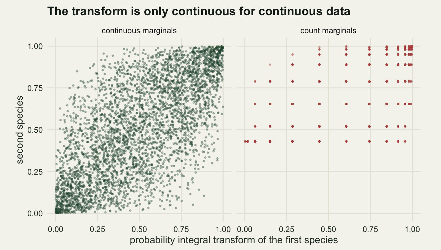
The backward direction is where it breaks. The probability integral transform of the count data takes only 17 distinct values across 4000 observations, and its largest deviation from a uniform is 0.1576, against 0.021 for the continuous case. The pseudo-observations are not uniform, they are a lattice, and Sklar’s uniqueness clause has gone with them: many different copulas reproduce the same joint distribution over the counts, because a copula is only pinned down at the corners of the lattice and is free in between. Genest and Neslehova (2007) work through what survives of the theory for count marginals and what does not. That is not a technicality about edge cases. It changes the answer to the question a reader will ask next, which is what the dependence between the two species actually is.
tau_conc <- function(x, y, blk = 400) {
  nn <- length(x)
  s <- 0
  for (i in seq(1, nn, by = blk)) {
    ix <- i:min(i + blk - 1, nn)
    s <- s + sum(sign(outer(x[ix], x, "-")) * sign(outer(y[ix], y, "-")))
  }
  s / (nn * (nn - 1))
}
tau_raw <- tau_conc(ya, yb)
tau_rb <- cor(ya, yb, method = "kendall")

set.seed(20260825)
tau_dt <- replicate(30, {
  w1 <- runif(n_sk)
  w2 <- runif(n_sk)
  cor(ppois(ya - 1, lam_p) + w1 * dpois(ya, lam_p),
      p_zip(yb - 1, zi_p, lam_z) +
        w2 * (p_zip(yb, zi_p, lam_z) - p_zip(yb - 1, zi_p, lam_z)),
      method = "kendall")
})
print(round(c(copula_tau = tau_set, concordance_tau = tau_raw,
              r_kendall_tau_b = tau_rb, distributional_transform = mean(tau_dt),
              dt_sd = sd(tau_dt), pearson = cor(ya, yb)), 4))
copula_tau concordance_tau r_kendall_tau_b
0.5000 0.4262 0.5241
distributional_transform dt_sd pearson
0.4261 0.0040 0.6524 Four numbers, one dataset, one generating copula whose tau is 0.5. Counting concordant minus discordant pairs and treating ties as neither gives 0.4262, an attenuation of 14.8 per cent caused entirely by the ties. What cor(method = "kendall") returns is tau-b, which divides by a tie-corrected denominator and overshoots in the other direction to 0.5241. Applying the distributional transform of Ruschendorf (2009), which spreads each atom uniformly over its own interval and does produce uniform margins, gives 0.4261 with a standard deviation of 0.004 across 30 draws of the randomisation. And Pearson’s correlation on the raw counts is 0.6524.
None of those four is wrong. They are answers to slightly different questions, and for continuous data they would collapse onto two, the copula tau and Pearson’s. For counts they do not collapse, and reporting “Kendall’s tau was 0.5241” without saying which estimator produced it hides a spread of 0.0978.
Three copulas, one Kendall’s tau
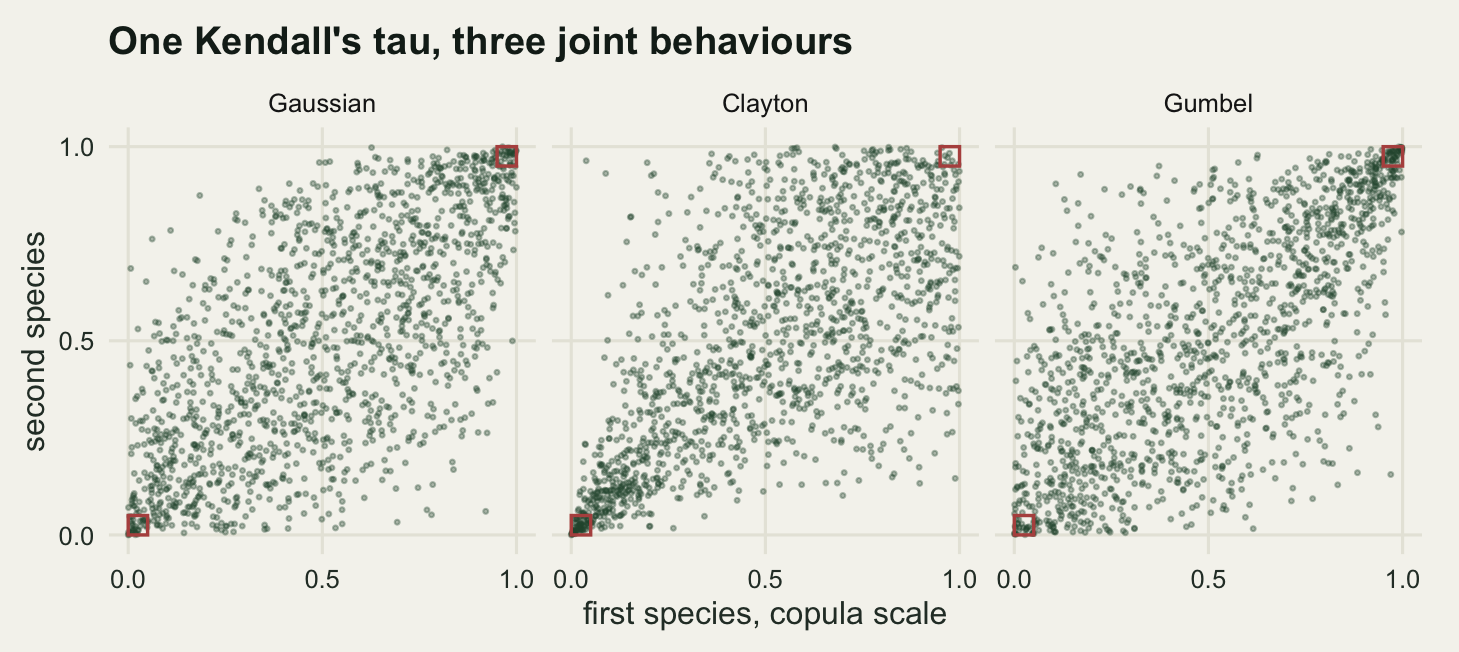
Return to continuous marginals and to the question the viability model was built for. Fix the two seabird marginals and fix Kendall’s tau at 0.5. There are still infinitely many joint distributions, and three of them are worth drawing.
The Gaussian copula is the one the Cholesky recipe produces. Clayton is asymmetric towards the lower tail: extreme low values arrive together far more often than extreme high ones. Gumbel is its mirror, asymmetric towards the upper tail. All three are set to the same population Kendall’s tau, land within a couple of hundredths of each other in Spearman’s rho, and carry exactly the same marginals.
set.seed(20260826)
n_sc <- 1500
sc_list <- list(Gaussian = draw_gauss(n_sc, rho_set),
                Clayton = draw_clay(n_sc, th_clay),
                Gumbel = draw_gum(n_sc, th_gum))
emp <- do.call(rbind, lapply(names(sc_list), function(nm) {
  s <- sc_list[[nm]]
  data.frame(family = nm, kendall = cor(s[, 1], s[, 2], method = "kendall"),
             spearman = cor(s[, 1], s[, 2], method = "spearman"))
}))
print(cbind(emp[, -1], family = emp$family), row.names = FALSE)
kendall spearman family
0.4807703 0.6690853 Gaussian
0.4971439 0.6748824 Clayton
0.5125657 0.6976737 Gumbelset.seed(20260828)
n_big <- 1e6
pearson_of <- function(uu) cor(qlnorm(uu[, 1], 0, sig_a), qlnorm(uu[, 2], 0, sig_b))
pear_tab <- c(gaussian = pearson_of(draw_gauss(n_big, rho_set)),
clayton = pearson_of(draw_clay(n_big, th_clay)),
gumbel = pearson_of(draw_gum(n_big, th_gum)))
pear_exact <- (exp(rho_set * sig_a * sig_b) - 1) /
sqrt((exp(sig_a^2) - 1) * (exp(sig_b^2) - 1))
print(round(c(pear_tab, gaussian_closed_form = pear_exact,
ratio_gumbel_clayton = unname(pear_tab["gumbel"] / pear_tab["clayton"])), 4)) gaussian clayton gumbel
0.4786 0.2109 0.6357
gaussian_closed_form ratio_gumbel_clayton
0.4639 3.0144 That is the first result of the section, and it is the mirror image of the opening. Three datasets with identical marginals and identical rank correlation report Pearson correlations of 0.2109, 0.4786 and 0.6357, a factor of 3.0144 between the smallest and the largest. The Gaussian entry has a closed form, 0.4639, so the Monte Carlo estimate at 1000000 draws is 0.0147 high, which is the accuracy to read the other two at. Pearson’s correlation is not a summary of the dependence. It is a summary of the dependence, the marginals and the interaction between them, and here the dependence shape alone moves it across most of its useful range.
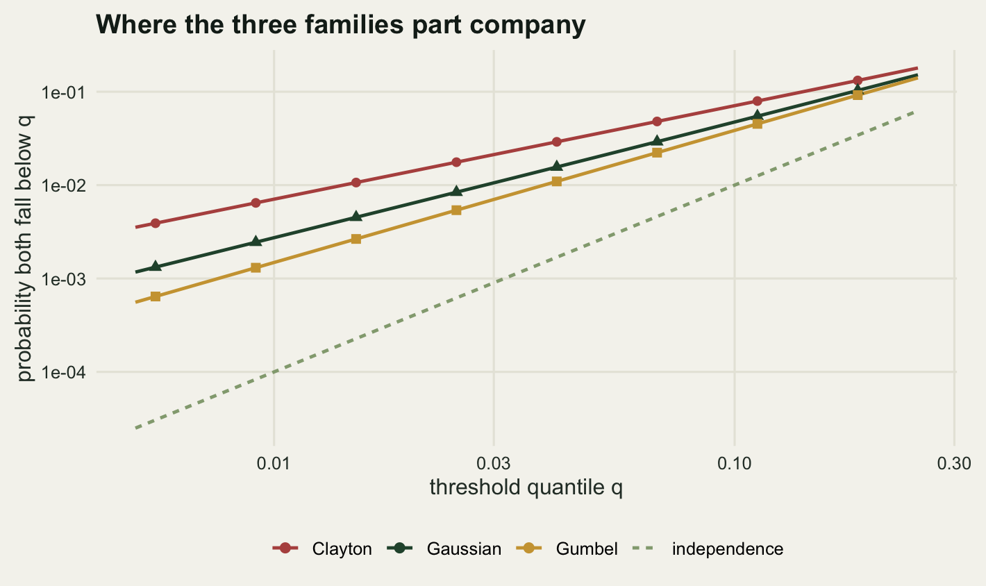
The second result is the one the conservation question needs. Joint exceedance probability is exactly what a copula computes: the probability that both species fall below their own q quantile in the same year is C(q, q), whatever the marginals are.
q_grid <- c(0.20, 0.10, 0.05, 0.02, 0.01)
tail_tab <- data.frame(q = q_grid, independent = q_grid^2,
                       gaussian = cop_gauss(q_grid, q_grid, rho_set),
                       clayton = cop_clay(q_grid, q_grid, th_clay),
                       gumbel = cop_gum(q_grid, q_grid, th_gum))
tail_tab$clay_over_gum <- tail_tab$clayton / tail_tab$gumbel
print(round(tail_tab, 6))
q independent gaussian clayton gumbel clay_over_gum
1 0.20 0.0400 0.113952 0.142857 0.102685 1.391217
2 0.10 0.0100 0.047386 0.070888 0.038529 1.839870
3 0.05 0.0025 0.019924 0.035377 0.014457 2.447152
4 0.02 0.0004 0.006410 0.014144 0.003956 3.574908
5 0.01 0.0001 0.002735 0.007071 0.001484 4.763465up_tab <- data.frame(q = q_grid,
gaussian = 1 - 2 * (1 - q_grid) +
cop_gauss(1 - q_grid, 1 - q_grid, rho_set),
clayton = 1 - 2 * (1 - q_grid) +
cop_clay(1 - q_grid, 1 - q_grid, th_clay),
gumbel = 1 - 2 * (1 - q_grid) +
cop_gum(1 - q_grid, 1 - q_grid, th_gum))
up_tab$gum_over_clay <- up_tab$gumbel / up_tab$clayton
print(round(up_tab, 6)) q gaussian clayton gumbel gum_over_clay
1 0.20 0.113952 0.085994 0.129371 1.504414
2 0.10 0.047386 0.025029 0.061567 2.459868
3 0.05 0.019924 0.006821 0.030029 4.402719
4 0.02 0.006410 0.001154 0.011833 10.254936
5 0.01 0.002735 0.000294 0.005887 20.016197Take a bad year for a species to be one in its worst five per cent. Under independence both species have a bad year together with probability 0.0025. Under the Gaussian copula it is 0.0199, under Gumbel 0.0145 and under Clayton 0.0354, so the Clayton world produces joint failures 2.447 times as often as the Gumbel world. Over the 30 years already monitored that is 1.061 expected joint failures against 0.434: roughly one that has already happened against one that probably has not. Sharpen the threshold to one year in a hundred and the ratio grows to 4.763.
The asymmetry runs the other way at the top. Both species having a top-one-per-cent year together has probability 0.005887 under Gumbel against 0.000294 under Clayton, a factor of 20.02. The Gaussian copula sits between the two in both tails and is symmetric between them, 0.002735 at the bottom and 0.002735 at the top, which is a property of the family rather than something the data asked for. Asymmetry of that kind is not hypothetical in ecological series: Ghosh et al (2020) survey cases where poor years associate more strongly with each other than good years do, and cases running the other way.
Fitting the three families, and telling them apart
The three pictures are different enough that a reader may reasonably expect the data to settle which one applies. Fitting is easy: take pseudo-observations from the ranks, which avoids committing to a marginal model at all, and maximise each copula’s log-likelihood over its single parameter. Genest and Favre (2007) set that rank-based procedure out step by step for practitioners. All three families have one parameter, so the AIC ranking is the log-likelihood ranking, and the AIC differences are twice the log-likelihood differences.
The dataset below is the monitoring scheme itself: 60 paired colony-years, generated from a Clayton copula at a Kendall’s tau of 0.5, with the two seabird marginals.
pobs <- function(x) rank(x) / (length(x) + 1)
fit3 <- function(u, v) {
  fg <- optimize(function(p) -sum(log(den_gauss(u, v, p))), c(-0.98, 0.98))
  fc <- optimize(function(p) -sum(log(den_clay(u, v, p))), c(0.02, 25))
  fu <- optimize(function(p) -sum(log(den_gum(u, v, p))), c(1.001, 15))
  ll <- -c(fg$objective, fc$objective, fu$objective)
  par <- c(fg$minimum, fc$minimum, fu$minimum)
  list(ll = ll, par = par, aic = -2 * ll + 2,
       tau = c(2 / pi * asin(par[1]), par[2] / (par[2] + 2), 1 - 1 / par[3]))
}
gen_cop <- function(fam, n, tau) {
  switch(fam,
         gaussian = draw_gauss(n, sin(pi * tau / 2)),
         clayton = draw_clay(n, 2 * tau / (1 - tau)),
         gumbel = draw_gum(n, 1 / (1 - tau)))
}

set.seed(20260827)
u_fit <- gen_cop("clayton", n_pair, tau_set)
fa <- qlnorm(u_fit[, 1], 0, sig_a)
fb <- qlnorm(u_fit[, 2], 0, sig_b)
ff <- fit3(pobs(fa), pobs(fb))
fit_tab <- data.frame(
  family = c("Gaussian", "Clayton", "Gumbel"),
  parameter = ff$par, implied_tau = ff$tau, loglik = ff$ll, aic = ff$aic,
  delta_aic = ff$aic - min(ff$aic),
  joint_low_1pct = c(cop_gauss(0.01, 0.01, ff$par[1]),
                     cop_clay(0.01, 0.01, ff$par[2]),
                     cop_gum(0.01, 0.01, ff$par[3])))
print(round(fit_tab[, -1], 5))
parameter implied_tau loglik aic delta_aic joint_low_1pct
1 0.54991 0.37068 9.22248 -16.44496 11.37395 0.00156
2 1.39448 0.41081 14.90945 -27.81891 0.00000 0.00609
3 1.46917 0.31935 5.93262 -9.86525 17.95366 0.00062print(fit_tab$family)[1] "Gaussian" "Clayton" "Gumbel" print(round(c(sample_kendall = cor(fa, fb, method = "kendall"),
sample_pearson = cor(fa, fb),
tau_spread_across_fits = diff(range(ff$tau)),
joint_low_ratio = max(fit_tab$joint_low_1pct) /
min(fit_tab$joint_low_1pct)), 5)) sample_kendall sample_pearson tau_spread_across_fits
0.38305 0.09970 0.09146
joint_low_ratio
9.77497 AIC picks the truth here, and by a clear margin: Clayton by 11.374 over the Gaussian copula and 17.954 over Gumbel. What the three fits agree on is the strength of the dependence. Their implied Kendall’s taus are 0.3707, 0.4108 and 0.3193, a spread of 0.0915, all of them near the sample value of 0.3831.
What they disagree on is the quantity the viability model exists to produce. The probability that both species have a one-in-a-hundred year together is 0.00609 under the fitted Clayton copula, 0.00156 under the fitted Gaussian one and 0.00062 under the fitted Gumbel: a ratio of 9.775 between the highest and the lowest, from three models fitted to the same sixty rows that agree on Kendall’s tau to within 0.0915.
One more number from the same dataset is the opening result reappearing. Pearson’s correlation on it is 0.0997 while Kendall’s tau is 0.3831. The Clayton copula puts its dependence in the lower tail, where the lognormal marginals are compressed, and takes it out of the upper tail where they are stretched, which is exactly the arrangement that makes a Pearson correlation small.
One dataset is one draw. The question that matters for practice is how often the ranking is right, and that needs a sweep over the true family, the sample size and the strength of the dependence.
sel_rate <- function(fam, n, tau, reps, seed) {
  set.seed(seed)
  pick <- integer(3)
  for (r in seq_len(reps)) {
    uu <- gen_cop(fam, n, tau)
    w <- which.min(fit3(pobs(uu[, 1]), pobs(uu[, 2]))$aic)
    pick[w] <- pick[w] + 1L
  }
  pick / reps
}

n_sel <- 600
grid_sel <- expand.grid(fam = c("gaussian", "clayton", "gumbel"),
                        n = c(60, 300), tau = c(0.25, 0.5),
                        stringsAsFactors = FALSE)
picks <- t(mapply(function(f, nn, tt, s) sel_rate(f, nn, tt, n_sel, s),
                  grid_sel$fam, grid_sel$n, grid_sel$tau,
                  20260830 + seq_len(nrow(grid_sel))))
colnames(picks) <- c("gaussian", "clayton", "gumbel")
sel_tab <- cbind(grid_sel, picks)
sel_tab$correct <- picks[cbind(seq_len(nrow(picks)),
                               match(grid_sel$fam, colnames(picks)))]
print(sel_tab, row.names = FALSE)
fam n tau gaussian clayton gumbel correct
gaussian 60 0.25 0.43000000 0.246666667 0.323333333 0.4300000
clayton 60 0.25 0.12333333 0.826666667 0.050000000 0.8266667
gumbel 60 0.25 0.19833333 0.085000000 0.716666667 0.7166667
gaussian 300 0.25 0.83166667 0.051666667 0.116666667 0.8316667
clayton 300 0.25 0.01666667 0.983333333 0.000000000 0.9833333
gumbel 300 0.25 0.07833333 0.001666667 0.920000000 0.9200000
gaussian 60 0.50 0.62333333 0.108333333 0.268333333 0.6233333
clayton 60 0.50 0.06500000 0.933333333 0.001666667 0.9333333
gumbel 60 0.50 0.17000000 0.020000000 0.810000000 0.8100000
gaussian 300 0.50 0.97333333 0.000000000 0.026666667 0.9733333
clayton 300 0.50 0.00000000 1.000000000 0.000000000 1.0000000
gumbel 300 0.50 0.02666667 0.000000000 0.973333333 0.9733333pick_at <- function(f, nn, tt, col = "correct") {
sel_tab[[col]][sel_tab$fam == f & sel_tab$n == nn & sel_tab$tau == tt]
}
print(round(c(worst_cell = min(sel_tab$correct),
best_cell = max(sel_tab$correct)), 4))worst_cell best_cell
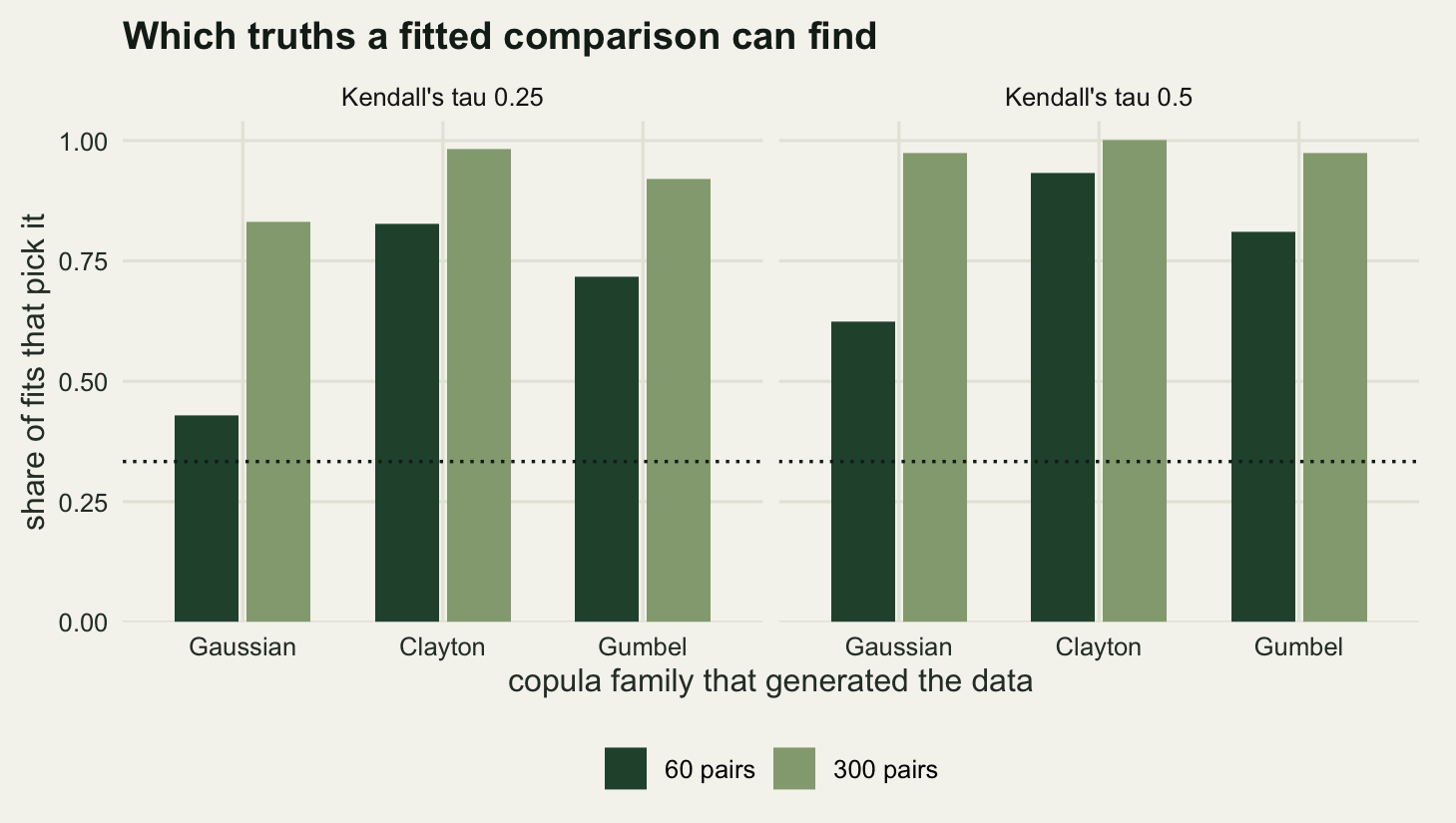
0.43 1.00 The difficulty is not uniform, and that was the surprise. The two asymmetric families are identifiable at monitoring-scale sample sizes: with 60 pairs and a tau of 0.25, a Clayton truth is recovered 82.7 per cent of the time and a Gumbel truth 71.7 per cent. The symmetric one is not. A Gaussian truth at the same sample size and the same tau is recovered 43 per cent of the time, with 32.3 per cent of the fits preferring Gumbel and 24.7 per cent preferring Clayton, which is not far from what three-sided guessing would give.
I expected all three to be hard to tell apart at 60 observations, and that is not what came out. The reason the asymmetric families are easier is that each has a feature the other two cannot imitate: a Clayton sample has a visible pinch in one corner, and neither of the others can produce it at any parameter value. A Gaussian sample has no such feature. It is the family without a signature, so any noisy sample from it can be read as a mild version of either asymmetric family, and 57 per cent of them are.
Raising the dependence helps the symmetric case a little: at a tau of 0.5 and 60 pairs, the Gaussian truth is recovered 62.3 per cent of the time. Raising the sample size helps far more: at 300 pairs and a tau of 0.25 it is 83.2 per cent, and the other five cells at that sample size all sit at or above 92 per cent. Three hundred paired observations is five colonies for sixty years, or sixty sites for five years. It is not out of reach, and it is a long way from thirty.
What to take away
Correlation is not a dial you can set. Choosing two marginals already fixes the interval of Pearson correlations that any joint distribution with those marginals can occupy, and for the two seabird marginals here that interval is -0.3094 to 0.7611. A viability model asking for 0.8 was asking for a distribution that does not exist. Push the second species’ skew a little further, to a log-scale standard deviation of 2.4, and the ceiling falls to 0.2751, so perfect monotone dependence would be reported as a weak correlation. Two Poisson species, one common at a mean of 20 and one rare at 0.2, cannot exceed 0.7201.
Spearman’s rho and Kendall’s tau have no such ceiling, reaching 1 and -1 on the couplings where Pearson reaches 0.7611 and -0.3094. That is not a reason to prefer them out of habit. It is the consequence of their depending on the copula alone, which is also why they are the right thing to specify when a simulation study needs a target.
The copula is what remains of a joint distribution once the marginals are divided out, and dividing them out is two lines: the probability integral transform forwards, a quantile function backwards. On a simulated dataset with continuous marginals that round trip recovered the copula parameter to 0.0036 and the marginals to 0.021 on the distribution-function scale, at 4000 observations.
Holding the marginals and Kendall’s tau fixed and changing only the copula family moved Pearson’s correlation from 0.2109 to 0.6357, and moved the probability that both species have a bottom-five-per-cent year together from 0.0145 to 0.0354. At the one-per-cent threshold the same three models differ by a factor of 4.763 in the lower tail and 20.02 in the upper. Three datasets a correlation coefficient would call identical carry joint-failure risks that differ by enough to change a management decision.
Two results went against what I expected. Distinguishing the families turned out to be easy for Clayton and Gumbel and hard for the Gaussian copula, rather than uniformly hard: 82.7 and 71.7 per cent correct at 60 pairs and a tau of 0.25, against 43 per cent for the Gaussian, whose fits scattered across the two asymmetric families. And the sample Pearson correlation of a heavily skewed pair turned out to sit far above its population value at monitoring sample sizes, with a median of 0.932 over 30 years where the population value is 0.7611, so the impossible target in the opening came from an estimator that was never estimating the bound.
The honest limits are three, and they compound. The copula is not identified separately from the marginals if the marginals are wrong: the pseudo-observations used above came from ranks, which is safe, but the moment a fitted parametric marginal is used for the transform, a misspecified marginal shows up as a distorted copula and nothing in the copula fit will say so. Rank-based pseudo-observations dodge that at the price of losing the marginals, which means the joint-exceedance probabilities above are statements about quantiles rather than about numbers of chicks.
Second, for discrete data the copula is not unique at all, because the probability integral transform is not continuous. Four defensible summaries of the same count dataset gave 0.4262, 0.5241, 0.4261 and 0.6524. The practical responses are to use the distributional transform and say that you did, since it at least produces uniform margins and a well-defined member of the compatible set, or to abandon the copula construction for counts and use a model that is discrete from the start, which is the route Joint species distribution models in R takes. Jittering the counts by a uniform is a third option and the worst of the three: it produces uniform margins by adding noise the data does not have, and the answer then depends on the jitter.
Third, the model-selection result is a floor rather than a ceiling on the difficulty. The sweep compared three families that were the only candidates and one of which was always correct. A real dataset is not generated by a Clayton copula, and a comparison among three wrong models will still return a winner with a comfortable AIC difference. A goodness-of-fit test asks the other question, whether a fitted family is compatible with the data at all, and Genest, Remillard and Beaudoin (2009) compare the power of the ones available. What the sweep does establish is that at 60 observations even the easy version of the problem, where the truth is on the list, fails 57 per cent of the time for the family that a Cholesky factor would have given you by default.
The tail behaviour that separated the three families has a formal name, the coefficient of tail dependence, and it is the quantity that decides whether joint extremes stay coupled as the threshold goes to the limit rather than merely at five or one per cent. That is the subject of tail dependence and joint extremes, which takes the same machinery into the far tail and puts a number on the joint-failure risk the viability model was after.
References
Sklar A 1959 Publications de l’Institut de Statistique de l’Universite de Paris 8:229-231
Nelsen RB 2006 An Introduction to Copulas, second edition (ISBN 978-0-387-28659-4)
Genest C, Favre AC 2007 Journal of Hydrologic Engineering 12(4):347-368 (10.1061/(ASCE)1084-0699(2007)12:4(347))
Genest C, Neslehova J 2007 ASTIN Bulletin 37(2):475-515 (10.2143/AST.37.2.2024077)
Demirtas H, Hedeker D 2011 The American Statistician 65(2):104-109 (10.1198/tast.2011.10090)
Ruschendorf L 2009 Journal of Statistical Planning and Inference 139(11):3921-3927 (10.1016/j.jspi.2009.05.030)
Genest C, Remillard B, Beaudoin D 2009 Insurance: Mathematics and Economics 44(2):199-213 (10.1016/j.insmatheco.2007.10.005)
Ghosh S, Sheppard LW, Holder MT, Loecke TD, Reid PC, Bever JD, Reuman DC 2020 Advances in Ecological Research 62:409-468 (10.1016/bs.aecr.2020.01.003)
Anderson MJ, de Valpine P, Punnett A, Miller AE 2019 Ecology and Evolution 9(6):3276-3294 (10.1002/ece3.4948)
Marshall AW, Olkin I 1988 Journal of the American Statistical Association 83(403):834-841 (10.1080/01621459.1988.10478671)