library(ggplot2)

te_pal <- list(forest = "#275139", green = "#2f8f63", sage = "#93a87f",
               clay = "#b5534e", gold = "#cda23f", line = "#dad9ca",
               ink = "#16241d", paper = "#f5f4ee")

theme_te <- function() {
  theme_minimal(base_size = 12) +
    theme(panel.grid.minor = element_blank(),
          panel.grid.major = element_line(colour = "#e7e6dc"),
          plot.background = element_rect(fill = "#f5f4ee", colour = NA),
          panel.background = element_rect(fill = "#f5f4ee", colour = NA),
          plot.title = element_text(face = "bold", colour = te_pal$ink),
          axis.title = element_text(colour = "#2c3a31"),
          axis.text = element_text(colour = "#2c3a31"))
}Tail dependence and joint extremes
R
extreme value theory
conservation
simulation
ecology tutorial
A correlation from the middle of a distribution says nothing about the corners. Simulating copulas in R to measure joint extreme risk in a reserve network.
Eight calcareous fens lie along one river catchment, each holding a population of the marsh fritillary, and each surveyed every September since the middle of the nineteen eighties by counting larval webs. A gauge at each fen logs the summer water deficit. Forty summers, eight sites, and the question the catchment partnership keeps asking is not about any one fen. It is whether the whole set can go under in the same year.
A bad summer at one fen is survivable. The webs disappear from that site and the fen fills in again over the following few years from a neighbour that was fine. A summer bad enough at every fen at once is a different event: nothing is left to recolonise from, and the network can be lost in a single year without any individual site having been more than ordinarily unlucky. The number the partnership needs is the annual probability of that joint event. Its two inputs are the site-level drought risk, which the gauge record supplies, and the dependence between the sites, which it does not.
Four posts here already treat the first input. Block maxima and the GEV fits a distribution to annual maxima, peaks over threshold keeps every exceedance instead of one per year, return levels and uncertainty puts an honest interval around the hundred-year event, and checking an extreme value model asks whether the fit deserves any of it. All four are univariate. None of them can reach the question above, because a return level for one fen says nothing whatever about what the fen four kilometres away is doing in the same summer, and no amount of extra care with the marginal fit will change that.
Dependence between populations is an old ecological subject under a different name. Liebhold, Koenig and Bjornstad (2004) review spatial synchrony, which arises from dispersal between populations, from a shared environmental driver (the Moran effect), or from predators and pathogens moving between sites; the measurement in that literature is almost always a correlation. The same question turns up in climate science as compound events, where Zscheischler and Seneviratne (2017) show that changing the dependence between two drivers moves the risk of the joint event far more than changing either driver on its own.
The dependence input is a copula question. Copulas for dependent ecological data builds the machinery, and closes on the observation that a Gaussian, a Clayton and a Gumbel copula tuned to the same Kendall’s tau put their mass in visibly different corners. This post takes that observation and makes it the whole subject, because in the corners is exactly where a reserve network lives or dies.
There is also a direct debt to SLOSS and reserve configuration, which ran the portfolio argument through a correlation coefficient and found the value at which several small stops beating single large. The addition here is that the interpolation between independent blocks and perfectly synchronised ones is not fixed by the correlation. Two networks can agree on every correlation you can measure and still differ by an order of magnitude in the probability that every block fails together, and the Gaussian assumption, which is what a multivariate normal simulation quietly imposes, sits at the optimistic end of that range.
Four measurements follow: the coefficient of tail dependence estimated and compared against theory for three copulas at one Kendall’s tau, the joint failure probability for the eight fens under each of them, the amount of data needed to tell the models apart, and the threshold at which a Gaussian copula finally admits to being asymptotically independent.
The quantity, and why correlation is not it
Write \(U\) and \(V\) for two variables mapped onto the unit interval by their own distribution functions, so that \(U\) is the quantile the first variable reached this year and \(V\) the quantile the second reached. The upper coefficient of tail dependence is
\[\lambda_U = \lim_{u \to 1} \Pr(V > u \mid U > u)\]
and the lower coefficient is the same construction at the other end, \(\lambda_L = \lim_{u \to 0} \Pr(V < u \mid U < u)\). In words: given that one site had a year in its worst one per cent, how often was the other site also in its worst one per cent, and what does that fraction settle down to as the threshold is pushed out. Sibuya (1960) wrote the quantity down; Coles, Heffernan and Tawn (1999) turned it into a diagnostic that gets used.
Two properties make it the right object. It is a function of the copula alone, so it does not move when the marginal distributions are rescaled, log transformed or replaced with something else entirely. And it is a statement about the corner rather than the middle, which a correlation coefficient never is. A Pearson correlation is an average over the whole joint distribution, and almost all of the mass it averages over sits nowhere near the tail.
The awkward part is that \(\lambda_U\) can be zero for a joint distribution that looks strongly dependent everywhere you can see. That case has a name, asymptotic independence, and Ledford and Tawn (1996) built the machinery for handling it. The Gaussian copula is the standard example, and it is also the default in every multivariate normal simulation an ecologist writes without thinking about it.
Three copulas at one Kendall’s tau
All three copulas used here can be generated the same way: draw one latent factor per year that all sites share, then draw one independent shock per site. That construction is what makes the simulation short and, later, what makes the risk probabilities available in closed form.
For the Gaussian copula with exchangeable correlation \(\rho\), the latent factor is a standard normal \(W\) and site \(i\) gets \(Z_i = \sqrt{\rho}\,W + \sqrt{1-\rho}\,\varepsilon_i\), pushed through the normal distribution function. For the two Archimedean copulas the factor is a positive random variable \(V\) acting as a frailty, and \(U_i\) is a decreasing function of an exponential shock divided by \(V\); Marshall and Olkin (1988) set this out in general. The Gumbel case needs \(V\) to be positive stable with index \(1/\theta\), which is where the Chambers, Mallows and Stuck (1976) algorithm comes in; the Clayton case needs only a gamma draw.
rcop_gauss <- function(n, d, rho) {
  z <- sqrt(rho) * matrix(rnorm(n), n, d) +
    sqrt(1 - rho) * matrix(rnorm(n * d), n, d)
  pnorm(z)
}

rstable_pos <- function(n, alpha) {
  w <- runif(n, 0, pi)
  ex <- rexp(n)
  (sin(alpha * w) / (sin(w))^(1 / alpha)) *
    (sin((1 - alpha) * w) / ex)^((1 - alpha) / alpha)
}

rcop_gumbel <- function(n, d, theta) {
  fr <- rstable_pos(n, 1 / theta)
  ex <- matrix(rexp(n * d), n, d)
  exp(-(ex / fr)^(1 / theta))
}

rcop_clayton <- function(n, d, theta) {
  fr <- rgamma(n, shape = 1 / theta, rate = 1)
  ex <- matrix(rexp(n * d), n, d)
  (1 + ex / fr)^(-1 / theta)
}
The three are matched on Kendall’s tau, which is a rank statistic and therefore a property of the copula rather than of the marginals. For a Gaussian copula \(\tau = (2/\pi)\arcsin\rho\); for Gumbel \(\tau = 1 - 1/\theta\); for Clayton \(\tau = \theta/(\theta + 2)\). Fix the Gaussian correlation, read off the tau, and invert the other two.
rho_base <- 0.8
tau_base <- 2 / pi * asin(rho_base)
th_gum <- 1 / (1 - tau_base)
th_clay <- 2 * tau_base / (1 - tau_base)

lam_gum_up <- 2 - 2^(1 / th_gum)
lam_clay_low <- 2^(-1 / th_clay)

set.seed(20260801)
n_tau <- 4000
tau_meas <- c(
  gaussian = cor(rcop_gauss(n_tau, 2, rho_base), method = "kendall")[1, 2],
  gumbel = cor(rcop_gumbel(n_tau, 2, th_gum), method = "kendall")[1, 2],
  clayton = cor(rcop_clayton(n_tau, 2, th_clay), method = "kendall")[1, 2])

print(round(c(rho = rho_base, kendall_tau = tau_base,
              gumbel_theta = th_gum, clayton_theta = th_clay,
              gumbel_upper_limit = lam_gum_up,
              clayton_lower_limit = lam_clay_low), 5))
rho kendall_tau gumbel_theta clayton_theta
0.80000 0.59033 2.44102 2.88203
gumbel_upper_limit clayton_lower_limit
0.67162 0.78623 print(round(tau_meas, 5))gaussian gumbel clayton
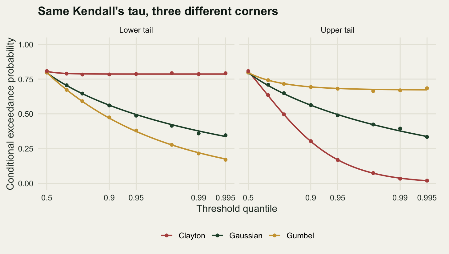
0.59497 0.59953 0.58500 A Gaussian correlation of 0.8 is a Kendall’s tau of 0.5903. That tau needs a Gumbel parameter of 2.441 and a Clayton parameter of 2.882, and the samplers reproduce it: 0.595, 0.5995 and 0.585 from 4000 draws each. Every rank-based summary a report would print about these three datasets agrees to within sampling error.
Their tail limits do not. The Gumbel copula has upper coefficient \(\lambda_U = 2 - 2^{1/\theta} =\) 0.6716 and lower coefficient zero. Clayton is the mirror image: lower coefficient \(2^{-1/\theta} =\) 0.7862 and upper coefficient zero. The Gaussian has zero at both ends for any correlation short of one.
Two of those are exact for every threshold, not only in the limit, because the diagonal of an Archimedean copula is a closed form. The Gaussian needs a one-dimensional integral, the inner normal probability integrated against the outer normal density.
lam_gauss_pex <- function(pex, rho) {
  ss <- sqrt(1 - rho^2)
  sapply(pex, function(pp) {
    zz <- qnorm(pp, lower.tail = FALSE)
    inner <- integrate(function(ee)
      exp(-zz * ee - ee^2 / 2) *
        pnorm((zz - rho * (zz + ee)) / ss, lower.tail = FALSE),
      0, Inf, rel.tol = 1e-10, subdivisions = 500L)$value
    dnorm(zz) * inner / pp
  })
}
lam_gauss_up <- function(uq, rho) lam_gauss_pex(1 - uq, rho)
lam_gum_up_at <- function(uq, theta) (1 - 2 * uq + uq^(2^(1 / theta))) / (1 - uq)
lam_gum_low_at <- function(uq, theta) (1 - uq)^(2^(1 / theta) - 1)
lam_clay_low_at <- function(uq, theta) {
  qq <- 1 - uq
  (2 * qq^(-theta) - 1)^(-1 / theta) / qq
}
lam_clay_up_at <- function(uq, theta) {
  cc <- (2 * uq^(-theta) - 1)^(-1 / theta)
  (1 - 2 * uq + cc) / (1 - uq)
}
uq_show <- c(0.5, 0.9, 0.95, 0.99, 0.995)
print(round(data.frame(
  threshold = uq_show,
  gauss_upper = lam_gauss_up(uq_show, rho_base),
  gumbel_upper = lam_gum_up_at(uq_show, th_gum),
  gumbel_lower = lam_gum_low_at(uq_show, th_gum),
  clayton_lower = lam_clay_low_at(uq_show, th_clay),
  clayton_upper = lam_clay_up_at(uq_show, th_clay)), 4))
threshold gauss_upper gumbel_upper gumbel_lower clayton_lower clayton_upper
1 0.500 0.7952 0.7964 0.7964 0.8056 0.8056
2 0.900 0.5624 0.6939 0.4695 0.7864 0.3022
3 0.950 0.4951 0.6827 0.3739 0.7863 0.1698
4 0.990 0.3769 0.6738 0.2204 0.7862 0.0377
5 0.995 0.3373 0.6727 0.1755 0.7862 0.0191The empirical estimator is a count. Rank each margin, convert to pseudo-observations, and take the fraction of the points above the threshold in one margin that are also above it in the other; Schmidt and Stadtmuller (2006) give its properties. Nothing about the estimator knows which copula generated the data.
lam_emp <- function(U, uq, tail) {
  n <- nrow(U)
  aa <- rank(U[, 1]) / (n + 1)
  bb <- rank(U[, 2]) / (n + 1)
  if (tail == "upper") {
    m <- sum(aa > uq)
    if (m == 0) return(NA_real_)
    sum(aa > uq & bb > uq) / m
  } else {
    qq <- 1 - uq
    m <- sum(aa < qq)
    if (m == 0) return(NA_real_)
    sum(aa < qq & bb < qq) / m
  }
}

set.seed(881204)
n_big <- 100000L
big_gauss <- rcop_gauss(n_big, 2, rho_base)
big_gum <- rcop_gumbel(n_big, 2, th_gum)
big_clay <- rcop_clayton(n_big, 2, th_clay)

uq_grid <- c(0.5, 0.7, 0.8, 0.9, 0.95, 0.98, 0.99, 0.995)
emp_tab <- data.frame(
  threshold = uq_grid,
  gauss_up = sapply(uq_grid, function(pt) lam_emp(big_gauss, pt, "upper")),
  gauss_low = sapply(uq_grid, function(pt) lam_emp(big_gauss, pt, "lower")),
  gum_up = sapply(uq_grid, function(pt) lam_emp(big_gum, pt, "upper")),
  gum_low = sapply(uq_grid, function(pt) lam_emp(big_gum, pt, "lower")),
  clay_up = sapply(uq_grid, function(pt) lam_emp(big_clay, pt, "upper")),
  clay_low = sapply(uq_grid, function(pt) lam_emp(big_clay, pt, "lower")))
print(round(emp_tab, 4))
threshold gauss_up gauss_low gum_up gum_low clay_up clay_low
1 0.500 0.7973 0.7973 0.7973 0.7973 0.8075 0.8075
2 0.700 0.7095 0.7055 0.7421 0.6728 0.6343 0.7892
3 0.800 0.6488 0.6458 0.7156 0.5909 0.4965 0.7827
4 0.900 0.5632 0.5605 0.6930 0.4743 0.3037 0.7834
5 0.950 0.4892 0.4872 0.6808 0.3800 0.1686 0.7866
6 0.980 0.4235 0.4145 0.6640 0.2775 0.0740 0.7925
7 0.990 0.3940 0.3590 0.6690 0.2150 0.0340 0.7860
8 0.995 0.3340 0.3460 0.6840 0.1700 0.0200 0.7920err_max <- max(abs(c(
emp_tab$gauss_up - lam_gauss_up(uq_grid, rho_base),
emp_tab$gum_up - lam_gum_up_at(uq_grid, th_gum),
emp_tab$clay_low - lam_clay_low_at(uq_grid, th_clay))))
n_deep <- n_big * (1 - max(uq_grid))
print(round(c(n = n_big, max_abs_error_vs_theory = err_max,
points_above_deepest_threshold = n_deep), 5)) n max_abs_error_vs_theory
1.00e+05 1.71e-02
points_above_deepest_threshold
5.00e+02 At 100000 draws the empirical curves sit within 0.0171 of the theoretical ones everywhere on the grid, including the deepest threshold where only 500 points are left to count. The estimator is doing its job, and any disagreement further on is a property of the models rather than of the code. At a threshold of 0.95 the Gaussian upper estimate is 0.4892, the Gumbel is 0.6808 and the Clayton is 0.1686. Push to 0.995 and the Gaussian has fallen to 0.334 while the Gumbel has barely moved, at 0.684 against its limit of 0.6716. The Clayton, which carries the strongest tail dependence of the three in the lower corner at 0.792, has almost nothing left in the upper one: 0.02.
Eight fens and one bad summer
Now the calculation the partnership wants. Call a summer bad at a fen if its water deficit lands in the worst 2 per cent of years for that fen, which is a one in fifty event locally. Nothing in what follows depends on the marginal distribution of the deficit: the threshold is defined by quantile, so the answer is a copula quantity from beginning to end.
Because all three copulas are one-factor constructions, the joint probability that every fen exceeds its threshold has a closed form. Conditional on the shared factor the sites are independent, so the probability is the expectation of a product. For the Gaussian that expectation is a one-dimensional integral over the latent normal. For the two Archimedean copulas an inclusion-exclusion expansion collapses onto the diagonal of the copula and gives a finite alternating sum, the Gumbel one being
\[\Pr(\text{all } d \text{ exceed } u) = \sum_{k=0}^{d} (-1)^k \binom{d}{k} u^{k^{1/\theta}}.\]
n_fen <- 8
p_bad <- 0.02

p_all_gauss <- function(pex, d, rho) {
  zz <- qnorm(pex, lower.tail = FALSE)
  integrate(function(w)
    dnorm(w) * pnorm((zz - sqrt(rho) * w) / sqrt(1 - rho), lower.tail = FALSE)^d,
    -Inf, Inf, rel.tol = 1e-12)$value
}
p_all_gum <- function(pex, d, theta) {
  uq <- 1 - pex
  kk <- 0:d
  sum((-1)^kk * choose(d, kk) * uq^(kk^(1 / theta)))
}
p_all_clay <- function(pex, d, theta) {
  uq <- 1 - pex
  kk <- 0:d
  sum((-1)^kk * choose(d, kk) * (1 + kk * (uq^(-theta) - 1))^(-1 / theta))
}

joint_now <- c(
  independent = p_bad^n_fen,
  clayton = p_all_clay(p_bad, n_fen, th_clay),
  gaussian = p_all_gauss(p_bad, n_fen, rho_base),
  gumbel = p_all_gum(p_bad, n_fen, th_gum))
print(signif(joint_now, 5))
independent clayton gaussian gumbel
2.5600e-14 1.1744e-07 1.9438e-03 9.3714e-03 ratio_gg <- joint_now[["gumbel"]] / joint_now[["gaussian"]]
ratio_span <- joint_now[["gumbel"]] / joint_now[["clayton"]]
d_eff <- log(joint_now) / log(p_bad)
print(round(d_eff, 4))independent clayton gaussian gumbel
8.0000 4.0790 1.5959 1.1938 print(round(c(gumbel_over_gaussian = ratio_gg, gumbel_over_clayton = ratio_span), 4))gumbel_over_gaussian gumbel_over_clayton
4.8211 79797.0071 Under independence the eight fens fail together with probability 2.56e-14, which is the number a planner gets by multiplying and which nobody believes. The three copulas, all agreeing on Kendall’s tau, give 1.174e-07 for Clayton, 0.001944 for Gaussian and 0.009371 for Gumbel. The Gumbel answer is 4.82 times the Gaussian one and 79,800 times the Clayton one.
The last of those is the wide number and the first is the useful one. Clayton is upper-tail independent, so as a model of joint drought it is the optimistic extreme in the same way independence is, only less obviously; if a copula were selected by eye from a scatterplot of the middle of the data and it happened to come out Clayton-shaped, the extrapolation to joint drought would be wrong by that whole factor. The Gaussian is the case that matters in practice, because it is what you get by default. Assuming it when the truth is Gumbel understates the joint risk by a factor of 4.82 at this threshold, with the same correlation in both.
A cleaner way to say the same thing is to ask how many independent fens the network is behaving like. Solve \(p^{d_{\text{eff}}}\) for the joint probability and read off the exponent.
horizon <- 50
p_horizon <- 1 - (1 - joint_now)^horizon
print(round(p_horizon, 6))
independent clayton gaussian gumbel
0.000000 0.000006 0.092703 0.375486 sloss_rho_star <- 0.6367 # crossover correlation from the SLOSS post
tau_star <- 2 / pi * asin(sloss_rho_star)
th_star <- 1 / (1 - tau_star)
four_g <- p_all_gauss(p_bad, 4, sloss_rho_star)
four_u <- p_all_gum(p_bad, 4, th_star)
print(round(c(tau = tau_star, gumbel_theta = th_star,
gumbel_upper_limit = 2 - 2^(1 / th_star)), 4)) tau gumbel_theta gumbel_upper_limit
0.4394 1.7838 0.5251 print(signif(c(gaussian_four = four_g, gumbel_four = four_u,
ratio = four_u / four_g,
deff_gaussian = log(four_g) / log(p_bad),
deff_gumbel = log(four_u) / log(p_bad)), 5))gaussian_four gumbel_four ratio deff_gaussian deff_gumbel
0.0013826 0.0077038 5.5719000 1.6830000 1.2439000 Eight fens behave like 1.596 independent ones under the Gaussian copula and like 1.194 under the Gumbel, against 8 under independence and 4.079 under Clayton. That is the portfolio benefit, and the choice of copula sets it: the Gaussian and Gumbel figures come from the same eight fens at the same correlation, so the whole gap between them is tail structure.
Over a 50 year planning horizon the annual probabilities compound into something a committee can act on: a 9.27 per cent chance of at least one total-failure summer under the Gaussian assumption against 37.55 per cent under the Gumbel. Those are different plans.
The SLOSS post put the crossover between four blocks and one at a correlation of 0.6367, the value above which splitting the reserve stops paying. At exactly that correlation, four blocks fail together with probability 0.001383 under a Gaussian copula and 0.007704 under a Gumbel one, a factor of 5.57. The crossover correlation is a real quantity and the post was right to chase it, but it is not sufficient: two catchments that agree on it can disagree by that factor on the event the reserve network exists to survive.
p_grid <- 10^seq(log10(0.2), log10(0.005), length.out = 25)
sweep_dat <- do.call(rbind, lapply(p_grid, function(pp) data.frame(
  pex = pp,
  Clayton = p_all_clay(pp, n_fen, th_clay),
  Gaussian = p_all_gauss(pp, n_fen, rho_base),
  Gumbel = p_all_gum(pp, n_fen, th_gum))))
sweep_dat$ratio <- sweep_dat$Gumbel / sweep_dat$Gaussian
print(round(sweep_dat[c(1, 9, 17, 25), ], 8))
pex Clayton Gaussian Gumbel ratio
1 0.20000000 0.01925199 0.05669596 0.10111780 1.783510
9 0.05848035 0.00008281 0.00904531 0.02782977 3.076707
17 0.01709976 0.00000004 0.00155804 0.00800324 5.136725
25 0.00500000 0.00000000 0.00028043 0.00232900 8.305228print(round(range(sweep_dat$ratio), 3))[1] 1.784 8.305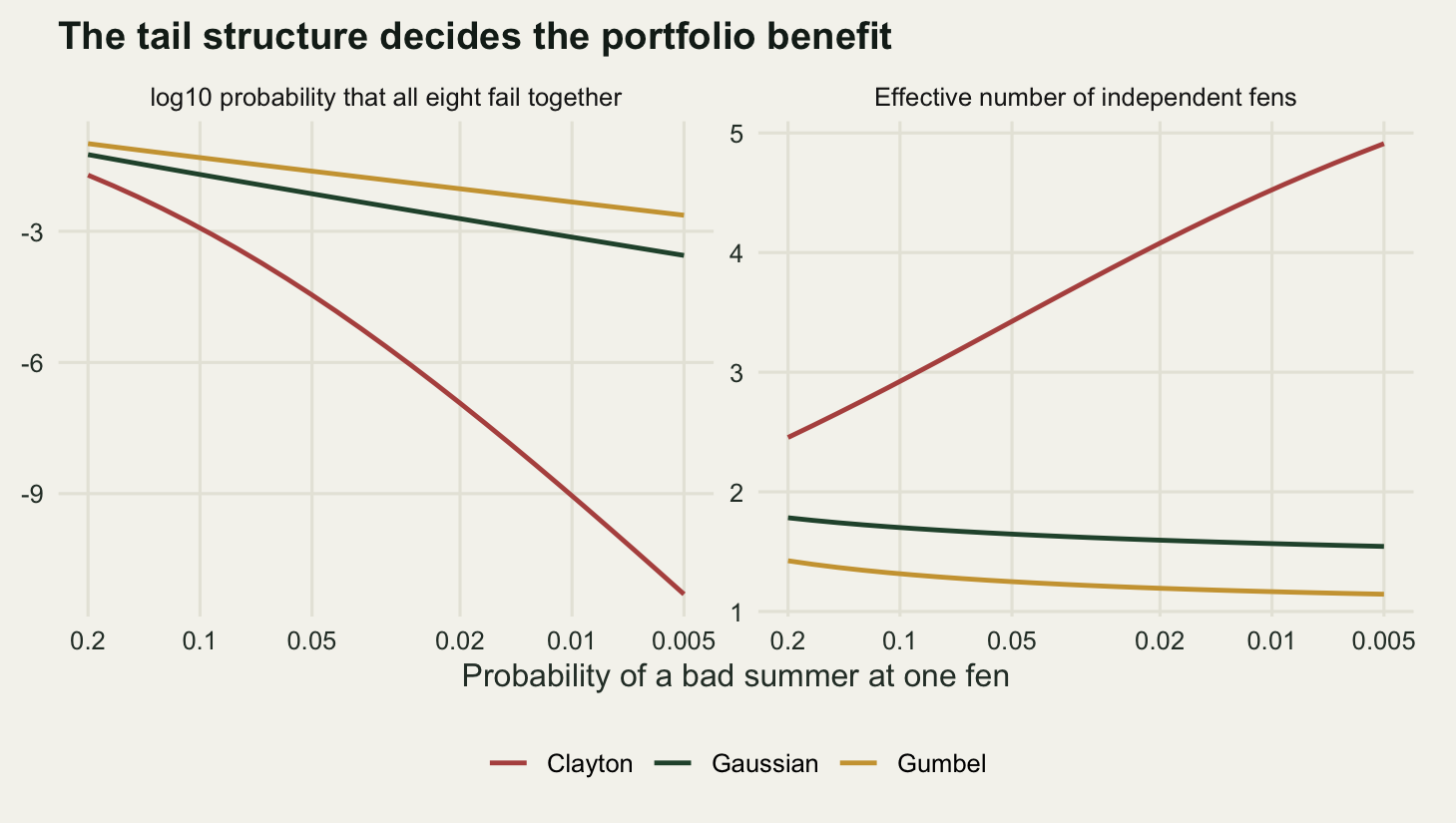
What it would take to see this in the data
The eight fens have forty summers of record. The obvious next move is to estimate the tail dependence coefficient from the data and let it decide between the models. This section measures whether that works.
Set the question up as a test. Under the null the truth is the Gaussian copula at correlation 0.8; under the alternative it is the Gumbel copula at the matching tau. Simulate many series of length \(n\) under each, compute the empirical coefficient at a threshold of 0.95, take the upper five per cent point of the null distribution as the critical value, and count how often the Gumbel case clears it.
uq_test <- 0.95
n_grid <- c(50, 100, 200, 400, 800, 1600, 3200)
n_rep_pow <- 2000

pow_np <- data.frame(n = n_grid, crit = NA_real_, power = NA_real_,
                     mean_null = NA_real_, mean_alt = NA_real_)
for (i in seq_along(n_grid)) {
  nn <- n_grid[i]
  set.seed(51000 + i)
  s_null <- replicate(n_rep_pow, lam_emp(rcop_gauss(nn, 2, rho_base), uq_test, "upper"))
  s_alt <- replicate(n_rep_pow, lam_emp(rcop_gumbel(nn, 2, th_gum), uq_test, "upper"))
  cv <- quantile(s_null, 0.95, na.rm = TRUE, names = FALSE)
  pow_np$crit[i] <- cv
  pow_np$power[i] <- mean(s_alt > cv, na.rm = TRUE)
  pow_np$mean_null[i] <- mean(s_null, na.rm = TRUE)
  pow_np$mean_alt[i] <- mean(s_alt, na.rm = TRUE)
}
print(round(pow_np, 4))
n crit power mean_null mean_alt
1 50 1.0000 0.0000 0.4360 0.6290
2 100 0.8000 0.0640 0.4753 0.6652
3 200 0.7000 0.2460 0.4830 0.6656
4 400 0.6500 0.5070 0.4938 0.6768
5 800 0.6000 0.8635 0.4918 0.6791
6 1600 0.5625 0.9975 0.4942 0.6798
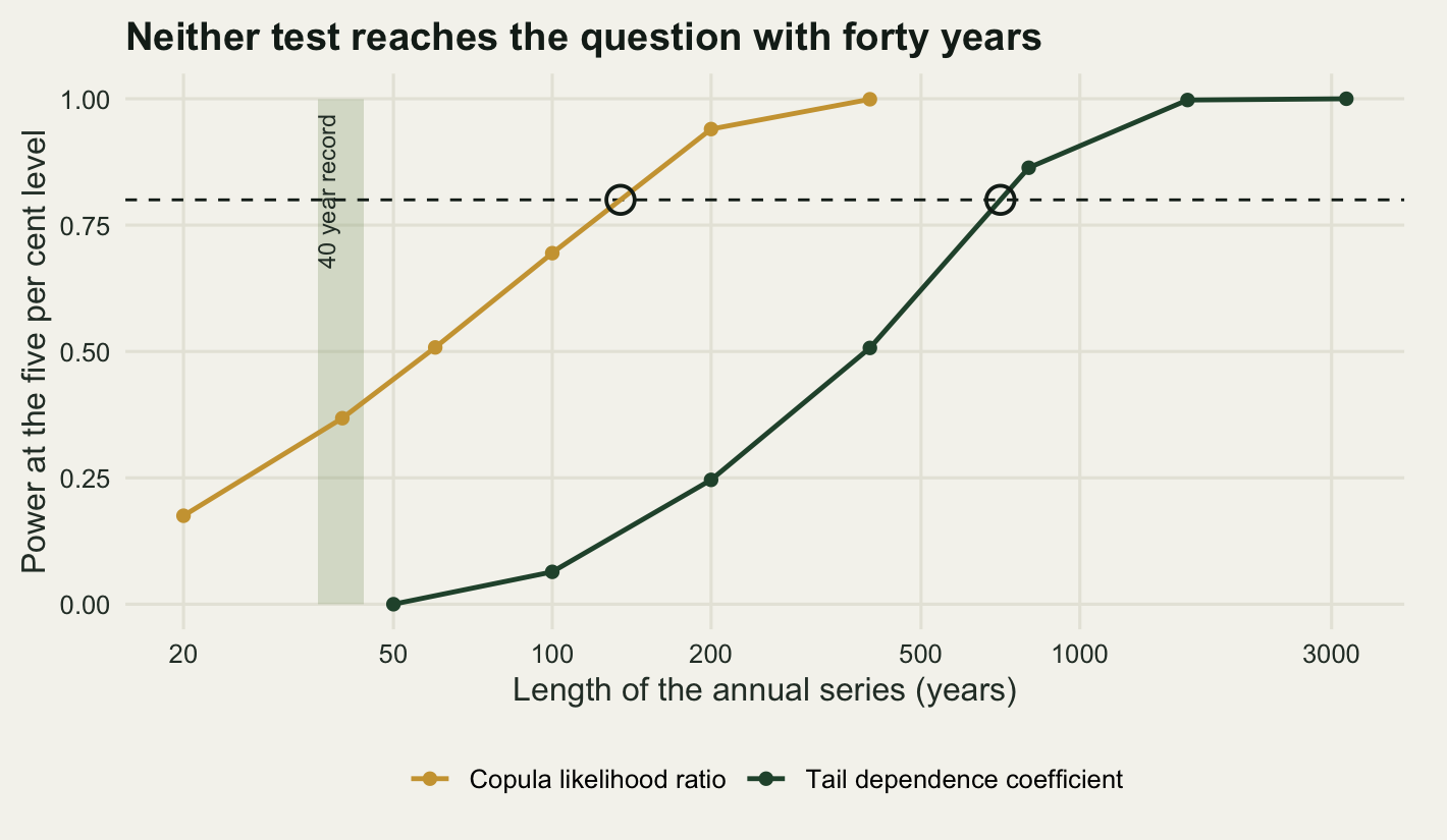
7 3200 0.5500 1.0000 0.4939 0.6825The two means separate immediately: 0.483 under the Gaussian against 0.6656 under the Gumbel at 200 years. The separation is not the problem. The spread is. At 200 years a threshold of 0.95 leaves 10 exceedances to estimate a proportion from, and the power is 0.246.
A parametric comparison should do better, because it uses every point rather than the ones in the corner. Both copulas have closed-form densities. Fit each by maximising the pseudo-likelihood over its single parameter, and use the difference in maximised log-likelihood as the statistic.
dens_gauss <- function(uu, vv, rho) {
  aa <- qnorm(uu); bb <- qnorm(vv)
  exp(-(rho^2 * (aa^2 + bb^2) - 2 * rho * aa * bb) / (2 * (1 - rho^2))) / sqrt(1 - rho^2)
}
dens_gumbel <- function(uu, vv, theta) {
  xx <- -log(uu); yy <- -log(vv)
  aa <- (xx^theta + yy^theta)^(1 / theta)
  exp(-aa) * (xx * yy)^(theta - 1) / (uu * vv) * aa^(1 - 2 * theta) * (aa + theta - 1)
}

lr_stat <- function(U) {
  n <- nrow(U)
  aa <- rank(U[, 1]) / (n + 1)
  bb <- rank(U[, 2]) / (n + 1)
  fg <- optimize(function(rr) sum(log(dens_gauss(aa, bb, rr))), c(0.01, 0.995),
                 maximum = TRUE)
  fu <- optimize(function(tt) sum(log(dens_gumbel(aa, bb, tt))), c(1.01, 25),
                 maximum = TRUE)
  fu$objective - fg$objective
}

n_grid_lr <- c(20, 40, 60, 100, 200, 400)
pow_lr <- data.frame(n = n_grid_lr, crit = NA_real_, power = NA_real_)
for (i in seq_along(n_grid_lr)) {
  nn <- n_grid_lr[i]
  set.seed(71000 + i)
  s_null <- replicate(n_rep_pow, lr_stat(rcop_gauss(nn, 2, rho_base)))
  s_alt <- replicate(n_rep_pow, lr_stat(rcop_gumbel(nn, 2, th_gum)))
  cv <- quantile(s_null, 0.95, names = FALSE)
  pow_lr$crit[i] <- cv
  pow_lr$power[i] <- mean(s_alt > cv)
}
print(round(pow_lr, 4))
n crit power
1 20 1.8163 0.1750
2 40 2.0800 0.3680
3 60 2.2075 0.5080
4 100 2.1544 0.6945
5 200 0.6788 0.9400
6 400 -5.1768 0.9990n80 <- function(tab) {
ok <- is.finite(tab$power)
approx(tab$power[ok], log(tab$n[ok]), xout = 0.8)$y
}
n80_np <- exp(n80(pow_np))
n80_lr <- exp(n80(pow_lr))
print(round(c(years_needed_coefficient = n80_np, years_needed_likelihood = n80_lr,
ratio = n80_np / n80_lr, record_length = 40), 1))years_needed_coefficient years_needed_likelihood ratio
707.1 134.7 5.2
record_length
40.0 Reaching eighty per cent power needs about 707 years of annual data from the coefficient and about 135 years from the likelihood ratio, a factor of 5.2 between them. The record is forty years. Neither number is within reach, and the first one is beyond any instrumental record: a 707 year run of parallel gauge records at eight fens does not exist and will not exist.
This is a finding rather than a shortfall in the analysis, and it has a practical consequence. Selecting a copula from the data is not available for this problem, so the choice has to come from somewhere else, which means from the mechanism. If the fens dry out because a blocking high sits over the whole catchment for six weeks, that is a shared driver that acts hardest in the worst years and the upper-tail-dependent model is the honest default. If they dry out because each fen’s own small aquifer happens to run low, tail independence is defensible. The second consequence is that a single number should not be reported. Run the calculation under both copulas and report the range: the numbers above show that range is a factor of 4.82 at the eight-fen threshold, which is small enough to state and large enough to matter.
The likelihood ratio deserves a caution as well. Its advantage comes entirely from assuming that one of the two candidate models is correct. When neither is, it selects whichever is closer in the middle of the data, where nearly all of the likelihood lives, and then hands over that model’s tail limit as though it had been estimated.
The threshold you can afford, and the one you would need
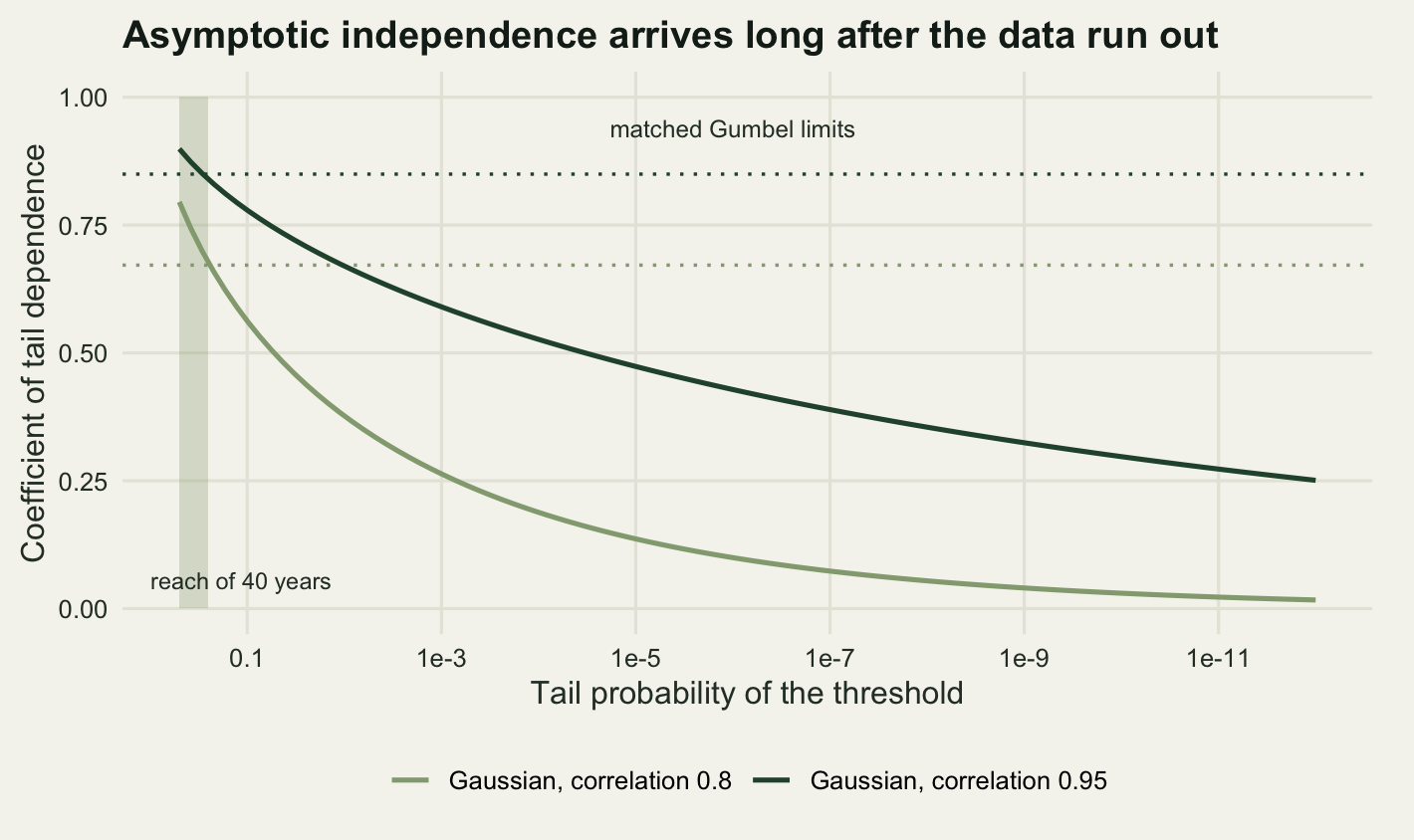
The Gaussian copula has zero tail dependence. Everything in the tables above says otherwise at every threshold anyone can estimate, and that is not a contradiction: the limit is approached, but slowly, and the approach happens outside the data.
Make the constraint explicit. Estimating a conditional exceedance probability needs some minimum number of points in the corner; take ten as a bare floor. A series of length \(n\) can then reach a threshold of \(u = 1 - 10/n\) and no further. Evaluate the exact Gaussian coefficient along that frontier.
rho_high <- 0.95
tau_high <- 2 / pi * asin(rho_high)
th_gum_high <- 1 / (1 - tau_high)
lam_gum_high <- 2 - 2^(1 / th_gum_high)

n_front <- 10^c(2, 3, 4, 6, 8, 12)
front <- data.frame(
  n = n_front,
  threshold = 1 - 10 / n_front,
  gauss_080 = lam_gauss_pex(10 / n_front, rho_base),
  gauss_095 = lam_gauss_pex(10 / n_front, rho_high))
print(format(front, digits = 4))
n threshold gauss_080 gauss_095
1 1e+02 0.900 0.56243 0.7792
2 1e+03 0.990 0.37690 0.6699
3 1e+04 0.999 0.26347 0.5901
4 1e+06 1.000 0.13635 0.4735
5 1e+08 1.000 0.07341 0.3892
6 1e+12 1.000 0.02257 0.2729need_n <- function(rho, target) {
f_root <- function(ln) lam_gauss_pex(10 / exp(ln), rho) - target
exp(uniroot(f_root, c(log(100), log(1e300)), tol = 1e-10)$root)
}
half_low <- lam_gum_up / 2
half_high <- lam_gum_high / 2
print(signif(c(rho_low_half_target = half_low,
years_rho_low = need_n(rho_base, half_low),
rho_high_half_target = half_high,
years_rho_high = need_n(rho_high, half_high),
years_rho_low_below_tenth = need_n(rho_base, 0.1),
years_rho_high_below_tenth = need_n(rho_high, 0.1)), 4)) rho_low_half_target years_rho_low
3.358e-01 2.059e+03
rho_high_half_target years_rho_high
4.248e-01 1.218e+07
years_rho_low_below_tenth years_rho_high_below_tenth
9.776e+06 7.950e+24 lam40 <- c(lam_gauss_pex(10 / 40, rho_base), lam_gauss_pex(10 / 40, rho_high))
print(round(c(gauss_080_at_40y = lam40[1], gauss_095_at_40y = lam40[2],
gumbel_limit_080 = lam_gum_up, gumbel_limit_095 = lam_gum_high), 4))gauss_080_at_40y gauss_095_at_40y gumbel_limit_080 gumbel_limit_095
0.6763 0.8393 0.6716 0.8496 At correlation 0.95 the picture is worse than at 0.8, and it is the more realistic case for sites in one catchment. The matched Gumbel copula has an upper limit of 0.8496. The Gaussian copula, whose limit is zero, reads 0.7792 at the frontier a hundred years of data can reach, 0.5901 at ten thousand years, and 0.2729 at a trillion. To get the estimate down to half the matched Gumbel value takes 12,200,000 years; to get it below 0.1 takes 7.95e+24 years, which is longer than the age of the universe by a wide margin.
At correlation 0.8 the same two questions want 2060 years and 9,780,000 years. The first of those is not absurd, and a paleoecological or tree-ring reconstruction could in principle reach it, which is worth knowing: the asymptotic behaviour of a moderate correlation is a millennium away rather than a cosmology away.
With the forty summers actually in hand the frontier is a threshold quantile of 0.75, where a Gaussian copula at 0.8 reads 0.6763 and one at 0.95 reads 0.8393. Both look like clear evidence of tail dependence, and the first of them is above the limit 0.6716 of the Gumbel copula it is being compared against, while the second is within 0.0103 of the Gumbel limit 0.8496. At the only threshold the record can reach, the asymptotically independent model looks about as tail dependent as the asymptotically dependent one, and their limits are as far apart as limits can be.
This is why the coefficient gets reported as comfortably positive from data generated by processes for which it is exactly zero, and it is not a mistake by whoever reported it: the estimate is close to unbiased for the quantity at the threshold used. The threshold is simply not the limit, and the distance between them is not crossable.
Honest limits
Everything above is bivariate or exchangeable. The tail dependence work is on pairs, and the eight-fen calculation gives every pair of fens the same dependence and every fen the same threshold. Real reserve networks are neither: fens sharing an aquifer will be locked together far more tightly than fens on opposite sides of a watershed, and the exchangeable answer will sit somewhere between the two subgroup answers without being right for either. Fitting a non-exchangeable structure means estimating a dependence parameter per pair, which is twenty-eight parameters here from forty years, and the data problem gets worse rather than better. Heffernan and Tawn (2004) give a conditional framework that scales past two variables without committing in advance to one regime or the other, and it is the right next step for anyone with more sites than this post handles.
The estimator conditions on rarer and rarer events, so its sampling error grows in exactly the region where the estimate carries the information. That is structural. A larger sample moves the frontier out but does not change the shape of the problem, which is why the years in the frontier table climb by powers of ten for each small step of the coefficient. No smoothing, bootstrap or bias correction fixes it, because there is no information there to correct.
The joint probabilities are exact for the copulas as written and say nothing about whether those copulas are right. A one-factor structure with a single shared driver per year is a modelling choice, and a catchment with a slow-moving drought front would want dependence that varies with lag as well as with distance. Autocorrelation is absent throughout: every year here is an independent draw, so the fifty-year horizon numbers are upper bounds on the chance of at least one total-failure summer, since a real sequence of dry summers arrives in runs.
Finally, the marginal side has been assumed away. The thresholds are quantiles of the true distribution, and in a real analysis they would come from a fitted GEV or GPD with the uncertainty the return level post documents at length. That uncertainty multiplies with the copula uncertainty measured here rather than replacing it.
References
Sibuya M 1960 Annals of the Institute of Statistical Mathematics 11(3):195-210 (10.1007/BF01682329)
Ledford AW, Tawn JA 1996 Biometrika 83(1):169-187 (10.1093/biomet/83.1.169)
Coles S, Heffernan J, Tawn J 1999 Extremes 2(4):339-365 (10.1023/A:1009963131610)
Heffernan JE, Tawn JA 2004 Journal of the Royal Statistical Society Series B 66(3):497-546 (10.1111/j.1467-9868.2004.02050.x)
Schmidt R, Stadtmuller U 2006 Scandinavian Journal of Statistics 33(2):307-335 (10.1111/j.1467-9469.2005.00483.x)
Marshall AW, Olkin I 1988 Journal of the American Statistical Association 83(403):834-841 (10.1080/01621459.1988.10478671)
Chambers JM, Mallows CL, Stuck BW 1976 Journal of the American Statistical Association 71(354):340-344 (10.1080/01621459.1976.10480344)
Zscheischler J, Seneviratne SI 2017 Science Advances 3(6):e1700263 (10.1126/sciadv.1700263)
Liebhold A, Koenig WD, Bjornstad ON 2004 Annual Review of Ecology Evolution and Systematics 35:467-490 (10.1146/annurev.ecolsys.34.011802.132516)