library(ggplot2)
library(patchwork)

te_paper  <- "#f5f4ee"
te_ink    <- "#16241d"
te_body   <- "#2c3a31"
te_forest <- "#275139"
te_rust   <- "#b5534e"
te_gold   <- "#c9b458"
te_line   <- "#dad9ca"

theme_datasheet <- function() {
  theme_minimal(base_size = 12) +
    theme(plot.background  = element_rect(fill = te_paper, colour = NA),
          panel.background = element_rect(fill = te_paper, colour = NA),
          panel.grid.major = element_line(colour = te_line, linewidth = 0.3),
          panel.grid.minor = element_blank(),
          text             = element_text(colour = te_body),
          plot.title       = element_text(colour = te_ink, face = "bold"),
          plot.subtitle    = element_text(colour = te_body),
          axis.text        = element_text(colour = te_body))
}Spatial synchrony and the Moran effect
R
population dynamics
time series
spatial synchrony
simulation
ecology tutorial
Shared weather gives populations its correlation only under narrow conditions, and dispersal synchrony depends on whether regulation cycles. Moran effect in R.
Sixteen moorland estates lie around the rim of one upland basin, and each has counted red grouse on the same transects every August for thirty years. The log counts of neighbouring estates rise and fall together. A report on the basin computes the correlation between every pair of estates, finds that it is highest for neighbours and falls away with distance, and then has to say why. There are two stock answers. The estates share the same weather, so a wet June depresses chick survival everywhere at once; or birds move between estates, so a good year on one spills into the next. The first is the Moran effect and the second is dispersal, and Liebhold, Koenig and Bjornstad (2004) list both, together with mobile predators and pathogens, as the standard causes of spatial synchrony.
The Moran effect also comes with a theorem, and the theorem is a number. Moran (1953), working on the Canadian lynx, observed that two populations governed by the same linear density dependence and disturbed by correlated noise should be correlated exactly as strongly as the noise. If that holds, the correlation between two estates is a direct measurement of the correlation between their weather, and nothing in the population dynamics needs to be known. This post measures when that equality holds, what breaks it, and whether the spatial pattern of synchrony can tell the Moran effect apart from dispersal.
The neighbour on this site is Tail dependence and joint extremes, which cites the same review and names the same mechanisms, but asks whether a correlation measured in the middle of a distribution says anything about joint failures in its corners. The question here is about the middle itself: whether the correlation of the populations is numerically the correlation of the environment. SLOSS and reserve configuration simulates Ricker populations with the environmental correlation set as an input and reads off persistence; this post asks what correlation of the populations such an input produces. The autoregressive coefficient used throughout is the Gompertz slope of Detecting density dependence in R, and the warning from Temporal autocorrelation and effective sample size, that autocorrelated series produce spurious correlations, reappears below as the width of the sampling distribution of a thirty year correlation.
The theorem and its conditions
Write the log abundance of population \(i\) as a deviation from its equilibrium, \(x_{i,t}\), and let it follow the Gompertz autoregression \(x_{i,t} = b_i x_{i,t-1} + \sigma \varepsilon_{i,t}\). The noise terms are independent from year to year, have unit variance, and are correlated between the two populations with correlation \(\rho\) in the same year. When \(|b_i| < 1\) the process is stationary and has variance \(\sigma^2 / (1 - b_i^2)\). The covariance between the two populations follows from the same recursion: it is \(\rho \sigma^2 / (1 - b_1 b_2)\). Dividing by the two standard deviations gives the correlation
\[\mathrm{cor}(x_1, x_2) = \rho \, \frac{\sqrt{(1 - b_1^2)(1 - b_2^2)}}{1 - b_1 b_2}.\]
When \(b_1 = b_2\) the fraction is exactly one and the population correlation equals the noise correlation. That is Moran’s theorem, and the derivation shows its conditions plainly. The two populations must have the same linear dynamics (the same coefficients; the result extends to any common linear autoregression of higher order). They must be stationary, so that the variances above exist. The noise must be correlated only within a year, not with a lag. And nothing may move between them. The noise variance does not have to be the same in the two populations, because it cancels in the correlation.
The fraction is never larger than one, so different density dependence can only lower synchrony below the noise correlation. The design constants below were fixed before any simulation was run: a noise correlation of 0.6, a noise standard deviation of 0.3 on the log scale, and a reference population with \(b_1 = 0.5\).
rho_env  <- 0.6      # correlation of the environmental noise
sd_env   <- 0.3      # noise standard deviation, log scale
b_ref    <- 0.5      # autoregressive (Gompertz) coefficient of the reference population
n_years  <- 30       # length of a realistic monitoring series

moran_cor <- function(b1, b2, rho) rho * sqrt((1 - b1^2) * (1 - b2^2)) / (1 - b1 * b2)

# many pairs at once: rows are replicate pairs, the loop runs over years
sim_ar_pair <- function(b1, b2, rho, n_rep, n_t, burn = 200, sig = sd_env) {
  x1 <- numeric(n_rep); x2 <- numeric(n_rep)
  s1 <- matrix(0, n_rep, n_t); s2 <- matrix(0, n_rep, n_t)
  for (k in seq_len(burn + n_t)) {
    z1 <- rnorm(n_rep)
    z2 <- rho * z1 + sqrt(1 - rho^2) * rnorm(n_rep)
    x1 <- b1 * x1 + sig * z1
    x2 <- b2 * x2 + sig * z2
    if (k > burn) { s1[, k - burn] <- x1; s2[, k - burn] <- x2 }
  }
  list(s1 = s1, s2 = s2)
}

row_cor <- function(m1, m2) {
  m1 <- m1 - rowMeans(m1); m2 <- m2 - rowMeans(m2)
  rowSums(m1 * m2) / sqrt(rowSums(m1^2) * rowSums(m2^2))
}
The closed form is a claim to check, so the check uses long series where sampling error is small: forty replicate pairs of five thousand years each, for five values of the second coefficient.
b_check  <- c(-0.5, 0, 0.5, 0.8, 0.95)
n_long   <- 5000
n_rep_lg <- 40
set.seed(5301)
check_tab <- do.call(rbind, lapply(b_check, function(b2) {
  pr <- sim_ar_pair(b_ref, b2, rho_env, n_rep_lg, n_long)
  rc <- row_cor(pr$s1, pr$s2)
  data.frame(b2 = b2, sim = mean(rc), se = sd(rc) / sqrt(n_rep_lg),
             theory = moran_cor(b_ref, b2, rho_env))
}))
check_tab$z <- (check_tab$sim - check_tab$theory) / check_tab$se
max_z <- max(abs(check_tab$z))
eq_sim <- check_tab$sim[check_tab$b2 == b_ref]
eq_se  <- check_tab$se[check_tab$b2 == b_ref]
cor_02_08 <- moran_cor(0.2, 0.8, rho_env)
cor_ref_95 <- moran_cor(b_ref, 0.95, rho_env)
cor_ref_neg <- moran_cor(b_ref, -0.5, rho_env)
round(check_tab, 3)
b2 sim se theory z
1 -0.50 0.358 0.001 0.360 -1.166
2 0.00 0.518 0.002 0.520 -0.913
3 0.50 0.602 0.002 0.600 1.148
4 0.80 0.518 0.002 0.520 -0.804
5 0.95 0.309 0.003 0.309 -0.069With identical coefficients the simulated correlation is 0.602 (Monte Carlo standard error 0.002) against a noise correlation of 0.6. Across all five second coefficients the simulated means sit within 1.2 standard errors of the closed form. The equality is exact where it is supposed to be, and the formula is right where it is not.
The losses are not small. A population with the reference coefficient paired with one close to a random walk, \(b_2 = 0.95\), has a correlation of 0.309 under the same weather. Pairing it with an overcompensating population, \(b_2 = -0.5\), gives 0.360. Two populations with coefficients 0.2 and 0.8 give 0.420. In each case the weather is identical and only the density dependence differs.
curve_df <- data.frame(b2 = seq(-0.95, 0.99, by = 0.01))
curve_df$cor <- moran_cor(b_ref, curve_df$b2, rho_env)

ggplot(curve_df, aes(b2, cor)) +
  geom_hline(yintercept = rho_env, linetype = "dashed", colour = te_rust, linewidth = 0.6) +
  geom_vline(xintercept = b_ref, colour = te_body, linetype = "dotted", linewidth = 0.7) +
  geom_line(colour = te_forest, linewidth = 1) +
  geom_errorbar(data = check_tab, aes(x = b2, ymin = sim - 2 * se, ymax = sim + 2 * se),
                inherit.aes = FALSE, width = 0.04, colour = te_ink, linewidth = 0.5) +
  geom_point(data = check_tab, aes(b2, sim), colour = te_ink, size = 2.2) +
  annotate("text", x = -0.9, y = rho_env + 0.025, label = "noise correlation",
           hjust = 0, colour = te_rust, size = 3.6) +
  scale_y_continuous(limits = c(0, 0.65)) +
  labs(x = "coefficient of the second population",
       y = "correlation of log abundance",
       title = "Equality only where the dynamics match",
       subtitle = "first population fixed at b = 0.5 (dotted line); bars: two Monte Carlo SE") +
  theme_datasheet()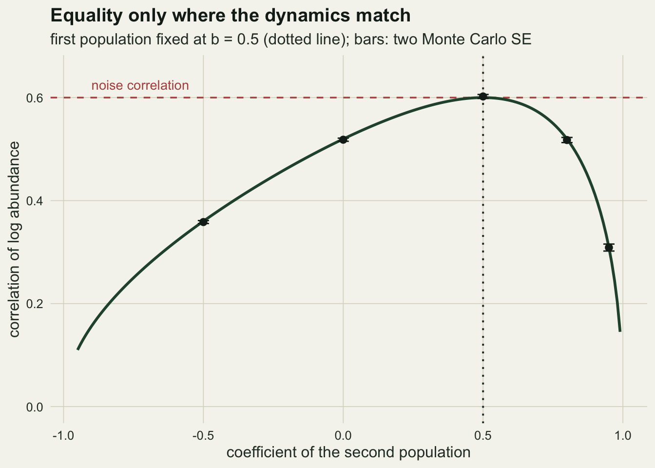
Thirty years is a short series
The theorem is about the process. A report has one thirty year series per estate and computes a sample correlation from it, and autocorrelated series make that estimate noisier than the same number of independent pairs would. The next chunk draws twenty thousand thirty year pairs with identical dynamics for three coefficients.
n_rep_sh <- 20000
b_short  <- c(0, 0.5, 0.8)
set.seed(7412)
short_list <- lapply(b_short, function(bb) {
  pr <- sim_ar_pair(bb, bb, rho_env, n_rep_sh, n_years)
  row_cor(pr$s1, pr$s2)
})
short_tab <- data.frame(b = b_short,
                        mean_r = vapply(short_list, mean, 0),
                        se_mean = vapply(short_list, function(v) sd(v) / sqrt(n_rep_sh), 0),
                        sd_r = vapply(short_list, sd, 0),
                        lo = vapply(short_list, function(v) quantile(v, 0.05), 0),
                        hi = vapply(short_list, function(v) quantile(v, 0.95), 0),
                        below_half = vapply(short_list, function(v) mean(v < rho_env / 2), 0))
iid_bias <- -rho_env * (1 - rho_env^2) / (2 * n_years)
# years of independent pairs that would give the same spread
n_equiv <- (1 - rho_env^2)^2 / short_tab$sd_r^2
round(short_tab, 3)
b mean_r se_mean sd_r lo hi below_half
1 0.0 0.594 0.001 0.123 0.368 0.770 0.022
2 0.5 0.590 0.001 0.152 0.310 0.802 0.046
3 0.8 0.577 0.002 0.229 0.132 0.866 0.125The mean sample correlation is 0.594 for independent years, 0.590 at \(b = 0.5\) and 0.577 at \(b = 0.8\), each with a Monte Carlo standard error of 0.0016 or less. For independent years the textbook first order bias of a sample correlation is \(-\rho(1 - \rho^2)/(2n)\), which here is -0.0064. The bias grows with autocorrelation, but it stays a matter of the second decimal place.
The spread does not. The standard deviation of the thirty year correlation is 0.123, 0.152 and 0.229 for the three coefficients, and the central ninety per cent interval at \(b = 0.8\) runs from 0.13 to 0.87. At that coefficient 12.5 per cent of pairs show a correlation below half the true noise correlation, where the theorem holds exactly. A single pair of estates cannot be used to read off the weather correlation; the equality is a statement about expectations. Using the large sample variance of a correlation from independent pairs, \((1 - \rho^2)^2 / n\), the spread at \(b = 0.8\) is what 7.8 independent years would give, against 27.1 for the white noise series of the same length.
short_df <- data.frame(r = unlist(short_list),
                       b = factor(rep(sprintf("b = %.1f", b_short), each = n_rep_sh),
                                  levels = sprintf("b = %.1f", b_short)))
ggplot(short_df, aes(r, colour = b)) +
  geom_density(linewidth = 1, adjust = 1.2) +
  geom_vline(xintercept = rho_env, linetype = "dashed", colour = te_rust, linewidth = 0.6) +
  scale_colour_manual(values = c(te_gold, te_forest, te_ink), name = NULL) +
  coord_cartesian(xlim = c(-0.5, 1)) +
  labs(x = "sample correlation over thirty years", y = "density",
       title = "Right on average, wide for any one pair",
       subtitle = "dashed red: the noise correlation, which is also the true synchrony") +
  theme_datasheet() +
  theme(legend.position = "bottom")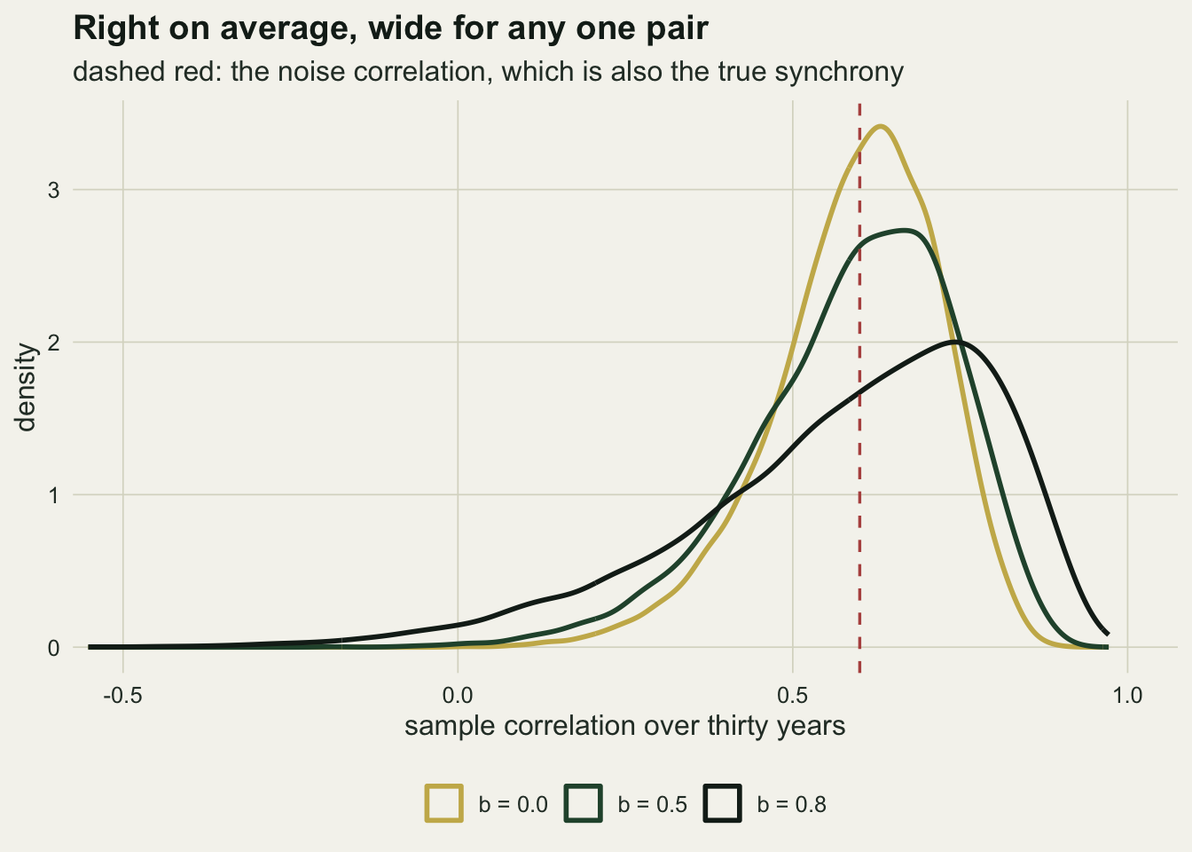
Dispersal on the same ring of estates
The second explanation needs a spatial layout, and a fair comparison needs the same layout for both. The sixteen estates sit on a ring, so every estate has two neighbours and distance is counted in steps around the ring. In the Moran scenario there is no movement and the noise correlation decays with distance as \(0.6^d\). In the dispersal scenario the noise is independent between estates, and each year the population first grows, then a fraction \(m = 0.05\) of each estate’s population moves, half to each neighbour, and only then does the year’s weather act. On the log scale and for small deviations the movement is a linear mixing step, so the whole ring is a multivariate autoregression \(x_t = b M x_{t-1} + \sigma \varepsilon_t\) with a mixing matrix \(M\). Its stationary covariance \(\Sigma\) solves \(\Sigma = (bM)\Sigma(bM)^\top + \sigma^2 C\), where \(C\) is the noise covariance matrix in units of \(\sigma^2\), and that linear equation can be solved exactly with a Kronecker product. The order of weather and movement is a modelling choice that matters here. If the weather acts before movement, part of each shock reaches the neighbours in the same year: the recursion becomes \(x_t = M(b x_{t-1} + \sigma \varepsilon_t)\), which has the same form with \(C = MM^\top\), and the chunk computes that variant too. (Whether growth comes before or after movement makes no difference, because a common scalar \(b\) commutes with \(M\).) The same coefficient and the same noise variance are used in both scenarios.
n_patch <- 16
m_disp  <- 0.05
ring_d  <- outer(seq_len(n_patch), seq_len(n_patch),
                 function(i, j) pmin(abs(i - j), n_patch - abs(i - j)))

mix_matrix <- function(m) {
  mm <- diag(1 - m, n_patch)
  for (i in seq_len(n_patch)) {
    mm[i, (i %% n_patch) + 1]     <- m / 2
    mm[i, ((i - 2) %% n_patch) + 1] <- m / 2
  }
  mm
}
stat_cov <- function(bmat, noise_cov) {
  np <- nrow(bmat)
  v  <- solve(diag(np * np) - kronecker(bmat, bmat), as.vector(noise_cov))
  matrix(v, np)
}
profile_by_d <- function(cmat) tapply(cmat, ring_d, mean)

noise_moran <- rho_env^ring_d
prof_moran  <- profile_by_d(cov2cor(stat_cov(diag(b_ref, n_patch), noise_moran)))
b_disp <- c(0.5, 0.8, 0.95)
prof_disp <- sapply(b_disp, function(bb)
  profile_by_d(cov2cor(stat_cov(bb * mix_matrix(m_disp), diag(n_patch)))))
noise_gap <- max(abs(prof_moran - rho_env^(0:(n_patch / 2))))
ratio_disp <- prof_disp[3, ] / prof_disp[2, ]
# weather before movement: each shock is partly shared with the neighbours in the same year
mm_disp <- mix_matrix(m_disp)
prof_pre <- sapply(b_disp, function(bb)
  profile_by_d(cov2cor(stat_cov(bb * mm_disp, mm_disp %*% t(mm_disp)))))
round(rbind(moran = prof_moran[2:5], t(prof_disp[2:5, ])), 3)
1 2 3 4
moran 0.600 0.360 0.216 0.130
0.015 0.000 0.000 0.000
0.073 0.006 0.001 0.000
0.248 0.065 0.017 0.004b_sweep <- seq(0, 0.98, by = 0.02)
nn_disp <- vapply(b_sweep, function(bb)
cov2cor(stat_cov(bb * mix_matrix(m_disp), diag(n_patch)))[1, 2], 0)
b_reach_third <- b_sweep[which(nn_disp >= 0.3)[1]]
n_above_third <- sum(nn_disp >= 0.3)
nn_max <- max(nn_disp)
nn_995 <- cov2cor(stat_cov(0.995 * mix_matrix(m_disp), diag(n_patch)))[1, 2]The Moran ring reproduces its noise profile at every distance, with a largest discrepancy that prints as 0.0000000000 at ten decimal places, so the theorem holds pair by pair on a network as long as the dynamics are identical. The dispersal ring is a different matter. With the reference coefficient, neighbouring estates reach a correlation of only 0.015; at \(b = 0.8\) it is 0.073, and at \(b = 0.95\) it is 0.248, against 0.60 for the Moran ring at distance one. If the weather acts before movement, the three values rise to 0.068, 0.125 and 0.297, so the timing changes the answer by a factor of up to 4.4, and the largest of the three is still 0.297. In this linear, stable model five per cent dispersal between neighbours does not produce synchrony as large as a noise correlation of 0.6 anywhere in the sweep below: even at \(b = 0.95\) neighbours reach 0.248, and the sweep reaches 0.406 only at its end, \(b =\) 0.98. Only a population very close to a random walk passes 0.6 (at \(b = 0.995\) neighbours reach 0.634). A strongly regulated linear population returns towards equilibrium quickly, and with it the deviation that each year’s immigrants brought in. That explanation belongs to linear dynamics; a later section shows that it fails once regulation overcompensates enough to cycle. Kendall and colleagues (2000) analysed a spatially structured population model with both mechanisms and report the same direction: synchrony falls as regulation strengthens, and dispersal and environmental correlation interact rather than add when both are present.
The shape of the decay differs too. Each step along the Moran profile multiplies the correlation by 0.60, by construction. The step from distance one to distance two multiplies the dispersal profile by 0.029, 0.086 and 0.261 for the three coefficients: with these constants, synchrony created by nearest neighbour dispersal is not only weaker but more local than synchrony created by a weather field decaying at 0.6 per step.
Sweeping the coefficient from 0 to 0.98 shows how strongly the answer depends on the dynamics. Neighbour synchrony from dispersal alone reaches 0.406 at the weakest density dependence on the grid. It exceeds 0.3 at 1 of the 50 grid values, the first being \(b =\) 0.98, a coefficient at which the population is close to a random walk and the stationary variance is large.
dist_show <- 1:6
prof_df <- rbind(
  data.frame(d = dist_show, sync = prof_moran[dist_show + 1], model = "shared noise, b = 0.5"),
  do.call(rbind, lapply(seq_along(b_disp), function(k)
    data.frame(d = dist_show, sync = prof_disp[dist_show + 1, k],
               model = sprintf("dispersal, b = %.2f", b_disp[k])))))
prof_df$model <- factor(prof_df$model, levels = unique(prof_df$model))

p_prof <- ggplot(prof_df, aes(d, sync, colour = model)) +
  geom_line(linewidth = 0.9) +
  geom_point(size = 2) +
  scale_y_log10(breaks = 10^seq(0, -10, by = -2),
                labels = parse(text = paste0("10^", seq(0, -10, by = -2)))) +
  scale_x_continuous(breaks = dist_show) +
  scale_colour_manual(values = c(te_rust, te_gold, te_forest, te_ink), name = NULL) +
  labs(x = "distance (steps around the ring)", y = "correlation (log scale)",
       title = "Weaker and more local") +
  theme_datasheet() +
  guides(colour = guide_legend(nrow = 2)) +
  theme(legend.position = "bottom")

sweep_df <- data.frame(b = b_sweep, sync = nn_disp)
p_sweep <- ggplot(sweep_df, aes(b, sync)) +
  geom_hline(yintercept = rho_env, linetype = "dashed", colour = te_rust, linewidth = 0.6) +
  geom_line(colour = te_forest, linewidth = 1) +
  scale_y_continuous(limits = c(0, 0.65)) +
  labs(x = "Gompertz coefficient b", y = "neighbour correlation",
       title = "Linear model: needs weak regulation") +
  theme_datasheet()

(p_prof | p_sweep) + plot_annotation(theme = theme_datasheet())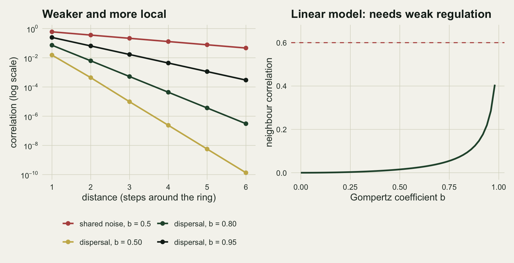
None of this means a distance profile can identify the mechanism. The theorem runs in reverse: any correlation profile a dispersal process produces is also produced by a Moran process whose noise correlation matrix equals that profile. The next chunk builds that impostor for the \(b = 0.95\) ring and compares two statistics a monitoring series offers beyond the lag zero correlation: each estate’s own lag one autocorrelation, and the neighbour cross-correlation at a lag of one year, which is where the two processes differ in principle. It also checks the exact covariance against a direct simulation of the dispersal ring.
b_hi <- 0.95
bmat_hi   <- b_hi * mix_matrix(m_disp)
cov_disp  <- stat_cov(bmat_hi, diag(n_patch))
cor_disp  <- cov2cor(cov_disp)
lag1_disp <- (bmat_hi %*% cov_disp)[1, 2] / cov_disp[1, 1]
acf1_disp <- (bmat_hi %*% cov_disp)[1, 1] / cov_disp[1, 1]

cov_imp  <- stat_cov(diag(b_hi, n_patch), cor_disp)
lag0_imp <- cov2cor(cov_imp)[1, 2]
lag1_imp <- (b_hi * cov_imp)[1, 2] / cov_imp[1, 1]

set.seed(9025)
n_ring_t <- 20000
x_ring <- numeric(n_patch)
ring_path <- matrix(0, n_ring_t, n_patch)
for (k in seq_len(n_ring_t + 500)) {
  x_ring <- as.vector(bmat_hi %*% x_ring) + rnorm(n_patch)
  if (k > 500) ring_path[k - 500, ] <- x_ring
}
ring_cor <- cor(ring_path)
sim_nn <- mean(ring_cor[ring_d == 1])
The simulated ring, 20000 years long, gives a mean neighbour correlation of 0.250 against the exact 0.248. The impostor matches the dispersal ring at lag zero by construction (0.248). Each estate’s own lag one autocorrelation is 0.914 in the dispersal ring and 0.95 in the impostor, whose estates are plain Gompertz series. At a lag of one year the dispersal ring has a neighbour cross-correlation of 0.249 and the impostor 0.236. Both differences are in the second decimal place, far inside the spread of a thirty year estimate measured in the previous section, so on count data alone the two mechanisms are indistinguishable here.
Nonlinear dynamics break the equality
The theorem needs linear density dependence, and real density dependence is not linear. The Ricker model on the log scale is \(x_{t+1} = x_t + r(1 - e^{x_t}) + \sigma\varepsilon_t\), with the carrying capacity scaled to one. Near equilibrium it behaves like a Gompertz model with coefficient \(1 - r\), so for \(0 < r < 2\) the linearisation is stationary and the theorem would predict a correlation of 0.6. At \(r = 2\) the deterministic model passes a period doubling and settles on a two year cycle. The chunk below runs both noise standard deviations, 0.1 and the reference 0.3, over a grid of growth rates, fifty replicate pairs of two thousand years each.
sim_ricker <- function(r_vals, sig, rho, n_rep, n_t, burn = 300) {
  rr <- rep(r_vals, each = n_rep); nn <- length(rr)
  x1 <- rep(0.05, nn); x2 <- rep(-0.05, nn)
  s1 <- matrix(0, nn, n_t); s2 <- matrix(0, nn, n_t)
  for (k in seq_len(burn + n_t)) {
    z1 <- rnorm(nn)
    z2 <- rho * z1 + sqrt(1 - rho^2) * rnorm(nn)
    x1 <- x1 + rr * (1 - exp(x1)) + sig * z1
    x2 <- x2 + rr * (1 - exp(x2)) + sig * z2
    if (k > burn) { s1[, k - burn] <- x1; s2[, k - burn] <- x2 }
  }
  data.frame(r = rr, cor = row_cor(s1, s2))
}

r_grid   <- seq(0.2, 2.8, by = 0.1)
sd_small <- 0.1
n_rep_rk <- 50
n_t_rk   <- 2000
set.seed(4460)
rk_tab <- do.call(rbind, lapply(c(sd_small, sd_env), function(sg) {
  out <- sim_ricker(r_grid, sg, rho_env, n_rep_rk, n_t_rk)
  data.frame(r = r_grid, sd = sg,
             sync = as.vector(tapply(out$cor, out$r, mean)),
             se = as.vector(tapply(out$cor, out$r, sd)) / sqrt(n_rep_rk))
}))
rk_at <- function(rv, sg) rk_tab[abs(rk_tab$r - rv) < 1e-9 & rk_tab$sd == sg, ]
rk_22_big <- rk_at(2.2, sd_env); rk_22_small <- rk_at(2.2, sd_small)
rk_15_big <- rk_at(1.5, sd_env); rk_15_small <- rk_at(1.5, sd_small)
rk_05_big <- rk_at(0.5, sd_env)
gap_05 <- rho_env - rk_05_big$sync
z_05 <- gap_05 / rk_05_big$se
z_15 <- (rho_env - rk_15_big$sync) / rk_15_big$se
At \(r = 0.5\) and the reference noise the Ricker pair has a correlation of 0.593 (standard error 0.003), which is 0.007 below the linear answer, or 2.4 standard errors: a trace of the nonlinearity, too small to matter against the sampling spread of any real series. At \(r = 1.5\), still below the period doubling, the two noise levels give 0.597 and 0.566: with small fluctuations the dynamics stay near the linear regime and the equality survives, while larger fluctuations reach the curvature of \(e^{x}\) and synchrony drops by a small amount that is still clearly real: 0.034, or 14 standard errors. At \(r = 2.2\) the two noise levels give 0.234 (standard error 0.020) and 0.361 (standard error 0.004).
That last pair of numbers runs against intuition. From \(r = 2.2\) upwards on this grid, the smaller noise gives the lower synchrony. The likely reason is phase. Two populations on a two year cycle can be in phase or out of phase, and the deterministic dynamics hold whichever phase they are in; it is the shared part of the noise that pushes them into step, and weak noise pushes weakly. Beyond the period doubling the correlation of the populations is no longer a property of the weather correlation alone, and the same weather can give very different synchrony depending on how large the fluctuations are. Grenfell and colleagues (1998) met the problem in real data: the Soay sheep on two islands of St Kilda fluctuate in close synchrony, and their nonlinear, threshold dynamics magnify random differences between the islands so much that only a high environmental correlation could explain the synchrony observed.
n_rep_rs <- 10000
set.seed(6118)
rs_out <- sim_ricker(c(0.5, 2.2), sd_env, rho_env, n_rep_rs, n_years)
rs_lin <- rs_out$cor[rs_out$r == 0.5]
rs_cyc <- rs_out$cor[rs_out$r == 2.2]
neg_lin <- mean(rs_lin < 0); neg_cyc <- mean(rs_cyc < 0)
In thirty year series at the reference noise, the Ricker pair at \(r = 2.2\) has a mean correlation of 0.361 with a standard deviation of 0.281, and 11.1 per cent of pairs are negatively correlated, against 0.19 per cent at \(r = 0.5\). Under a shared weather field with a correlation of 0.6, an estate pair that looks independent or even opposed is not rare for a cycling population: about one pair in 9.
rk_tab$noise <- factor(sprintf("noise sd %.1f", rk_tab$sd),
                       levels = sprintf("noise sd %.1f", c(sd_small, sd_env)))
ggplot(rk_tab, aes(r, sync, colour = noise)) +
  geom_hline(yintercept = rho_env, linetype = "dashed", colour = te_rust, linewidth = 0.6) +
  geom_vline(xintercept = 2, linetype = "dotted", colour = te_body, linewidth = 0.6) +
  geom_errorbar(aes(ymin = sync - 2 * se, ymax = sync + 2 * se), width = 0.04, linewidth = 0.5) +
  geom_line(linewidth = 0.9) +
  geom_point(size = 1.6) +
  scale_colour_manual(values = c(te_gold, te_forest), name = NULL) +
  scale_x_continuous(breaks = seq(0, 3, by = 0.5)) +
  coord_cartesian(ylim = c(0, 0.7)) +
  labs(x = "Ricker growth rate r", y = "correlation of log abundance",
       title = "The equality fails where the dynamics bend",
       subtitle = "dashed red: noise correlation; bars: two Monte Carlo SE") +
  theme_datasheet() +
  theme(legend.position = "bottom")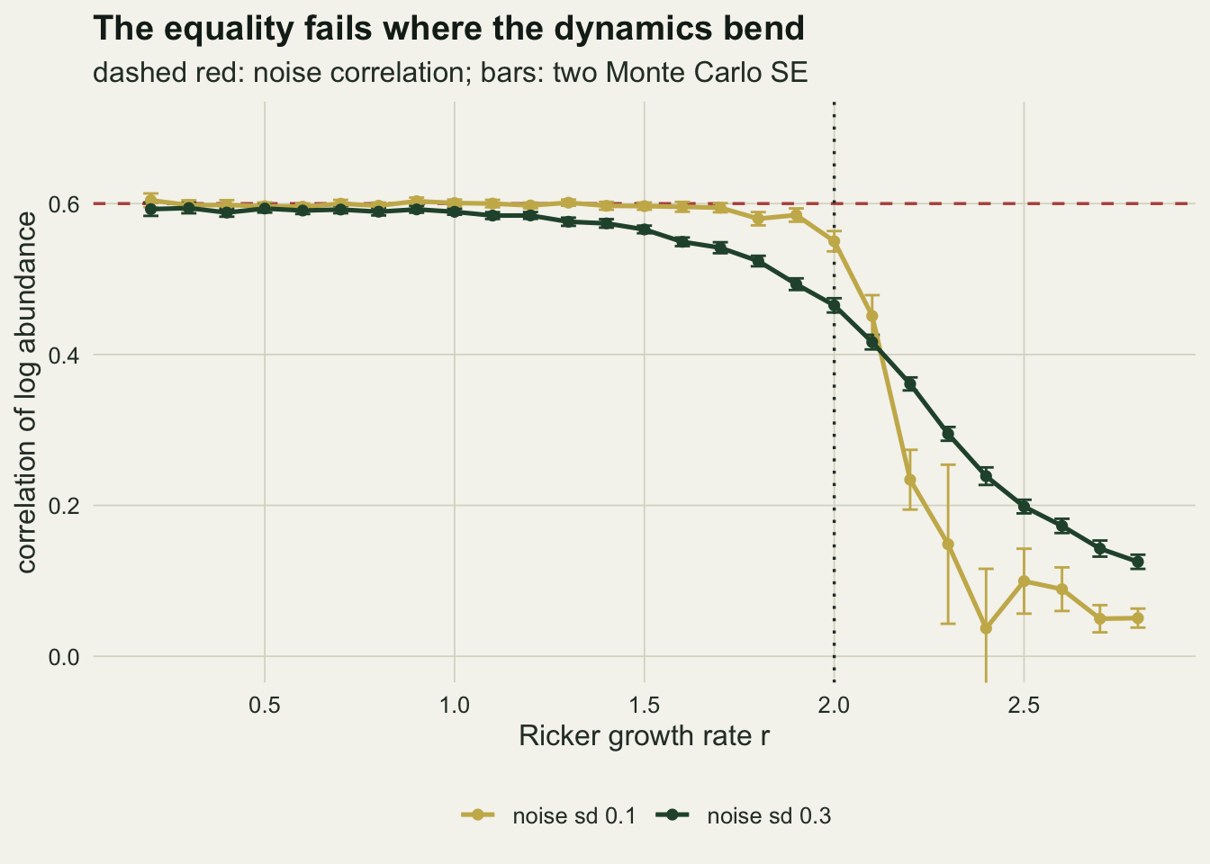
Dispersal in a cycling ring
The dispersal section above used linear, stable dynamics, and its conclusion, that strong regulation leaves little room for dispersal to synchronise, was drawn from that model. The Ricker model can overcompensate without cycling (for \(1 < r < 2\) its linearisation has a negative coefficient) and cycles beyond \(r = 2\), so it tests whether the conclusion is about the strength of regulation or about its form. The chunk below puts sixteen Ricker estates on the same ring with independent noise and moves five per cent of the individuals each year, half to each neighbour, on the natural scale rather than the log scale, so no small deviation approximation is involved. The order matches the linear ring: growth, then movement, then the year’s weather. Twelve replicate rings of three thousand years are run for each growth rate on the grid of the previous section and for both noise levels, and at \(r = 2.2\) the order with the weather before movement is run as well.
sim_ricker_ring <- function(rr, sig, n_rep, n_t, burn = 500, noise_first = FALSE) {
  x <- matrix(rnorm(n_rep * n_patch, 0, 0.1), n_rep)
  path <- array(0, c(n_rep, n_t, n_patch))
  for (k in seq_len(burn + n_t)) {
    eps <- sig * matrix(rnorm(n_rep * n_patch), n_rep)
    if (noise_first) {
      x <- log(exp(x + rr * (1 - exp(x)) + eps) %*% mm_disp)
    } else {
      x <- log(exp(x + rr * (1 - exp(x))) %*% mm_disp) + eps
    }
    if (k > burn) path[, k - burn, ] <- x
  }
  cors <- lapply(seq_len(n_rep), function(i) cor(path[i, , ]))
  list(nn = vapply(cors, function(cm) mean(cm[ring_d == 1]), 0),
       d2 = vapply(cors, function(cm) mean(cm[ring_d == 2]), 0))
}

n_rep_ring <- 12
n_t_ring   <- 3000
set.seed(2718)
ring_tab <- do.call(rbind, lapply(c(sd_small, sd_env), function(sg) {
  do.call(rbind, lapply(r_grid, function(rv) {
    out <- sim_ricker_ring(rv, sg, n_rep_ring, n_t_ring)
    data.frame(r = rv, sd = sg, sync = mean(out$nn),
               se = sd(out$nn) / sqrt(n_rep_ring), d2 = mean(out$d2))
  }))
}))
ring_pre <- vapply(c(sd_small, sd_env), function(sg)
  mean(sim_ricker_ring(2.2, sg, n_rep_ring, n_t_ring, noise_first = TRUE)$nn), 0)
ring_at <- function(rv, sg) ring_tab[abs(ring_tab$r - rv) < 1e-9 & ring_tab$sd == sg, ]
rg_small <- ring_tab[ring_tab$sd == sd_small, ]
rg_big   <- ring_tab[ring_tab$sd == sd_env, ]
rg_02 <- ring_at(0.2, sd_env); rg_05 <- ring_at(0.5, sd_small); rg_15 <- ring_at(1.5, sd_small)
rg_22s <- ring_at(2.2, sd_small); rg_22b <- ring_at(2.2, sd_env)
rg_28s <- ring_at(2.8, sd_small)
rg_peak <- rg_small[which.max(rg_small$sync), ]
lin_08 <- cov2cor(stat_cov(0.8 * mm_disp, diag(n_patch)))[1, 2]
max_se_ring <- max(ring_tab$se)
round(ring_tab[ring_tab$r >= 1.9, ], 3)
r sd sync se d2
18 1.9 0.1 0.099 0.003 0.010
19 2.0 0.1 0.175 0.004 0.034
20 2.1 0.1 0.332 0.005 0.115
21 2.2 0.1 0.562 0.009 0.325
22 2.3 0.1 0.627 0.016 0.382
23 2.4 0.1 0.412 0.021 0.128
24 2.5 0.1 -0.045 0.017 0.005
25 2.6 0.1 -0.419 0.024 0.246
26 2.7 0.1 -0.598 0.021 0.402
27 2.8 0.1 -0.766 0.030 0.665
45 1.9 0.3 0.040 0.002 0.003
46 2.0 0.3 0.048 0.002 0.000
47 2.1 0.3 0.054 0.002 0.004
48 2.2 0.3 0.064 0.003 0.004
49 2.3 0.3 0.068 0.001 0.002
50 2.4 0.3 0.069 0.003 0.002
51 2.5 0.3 0.062 0.003 0.001
52 2.6 0.3 0.046 0.003 -0.003
53 2.7 0.3 0.032 0.003 0.004
54 2.8 0.3 0.007 0.002 0.012Well below the period doubling the ring behaves like the linear model. At \(r = 0.2\), whose linearisation has \(b = 0.8\), neighbours reach 0.073 at the reference noise against the exact linear 0.073. With the small noise, \(r = 0.5\) and \(r = 1.5\), whose linearisations have coefficients of the same size and opposite sign, give 0.015 and 0.012; in the linear model a sign change of \(b\) leaves the stationary correlation unchanged, so overcompensation that does not cycle adds nothing. The largest Monte Carlo standard error anywhere in the table is 0.030.
Past \(r = 2\) with the small noise the picture reverses. Neighbour synchrony climbs to 0.562 at \(r = 2.2\) and 0.627 at \(r =\) 2.3 (standard error 0.016), the size of the weather correlation used for the Moran scenario, from independent weather and the same five per cent movement that gave almost nothing in the linear ring. Regulation here is stronger, not weaker, than anywhere in the linear sweep. What dispersal does to a cycling population is not to carry deviations that density dependence then erases; it nudges the phase of each two year cycle towards its neighbours, and a small nudge each year is enough to hold neighbours in step. At \(r = 2.2\) that is more neighbour synchrony than a weather correlation of 0.6 gave two isolated Ricker populations with the same small noise in the previous section (0.234), although a ring and a pair are not strictly the same comparison. Further out the locking changes sign: at \(r = 2.8\) neighbours are correlated at -0.766 and estates two steps apart at 0.665, an alternating pattern around the ring in which estates tend to be high when their neighbours are low. With the reference noise the locking never forms: the largest neighbour correlation on the whole grid is 0.073, and at \(r = 2.2\) it is 0.064. Letting the weather act before movement raises the two \(r = 2.2\) values to 0.627 and 0.103 and does not change the pattern.
So the strength of dispersal synchrony is not a function of the strength of regulation alone. It depends on the form of the dynamics, and in the cycling ring also on the size of the noise that competes with the locking.
ring_tab$noise <- factor(sprintf("noise sd %.1f", ring_tab$sd),
                         levels = sprintf("noise sd %.1f", c(sd_small, sd_env)))
ggplot(ring_tab, aes(r, sync, colour = noise)) +
  geom_hline(yintercept = rho_env, linetype = "dashed", colour = te_rust, linewidth = 0.6) +
  geom_hline(yintercept = 0, colour = te_body, linewidth = 0.4) +
  geom_vline(xintercept = 2, linetype = "dotted", colour = te_body, linewidth = 0.6) +
  geom_errorbar(aes(ymin = sync - 2 * se, ymax = sync + 2 * se), width = 0.04, linewidth = 0.5) +
  geom_line(linewidth = 0.9) +
  geom_point(size = 1.6) +
  scale_colour_manual(values = c(te_gold, te_forest), name = NULL) +
  scale_x_continuous(breaks = seq(0, 3, by = 0.5)) +
  coord_cartesian(ylim = c(-0.85, 0.75)) +
  labs(x = "Ricker growth rate r", y = "neighbour correlation",
       title = "Dispersal locks cycles when the noise is small",
       subtitle = "independent noise; dashed red: 0.6; bars: two Monte Carlo SE") +
  theme_datasheet() +
  theme(legend.position = "bottom")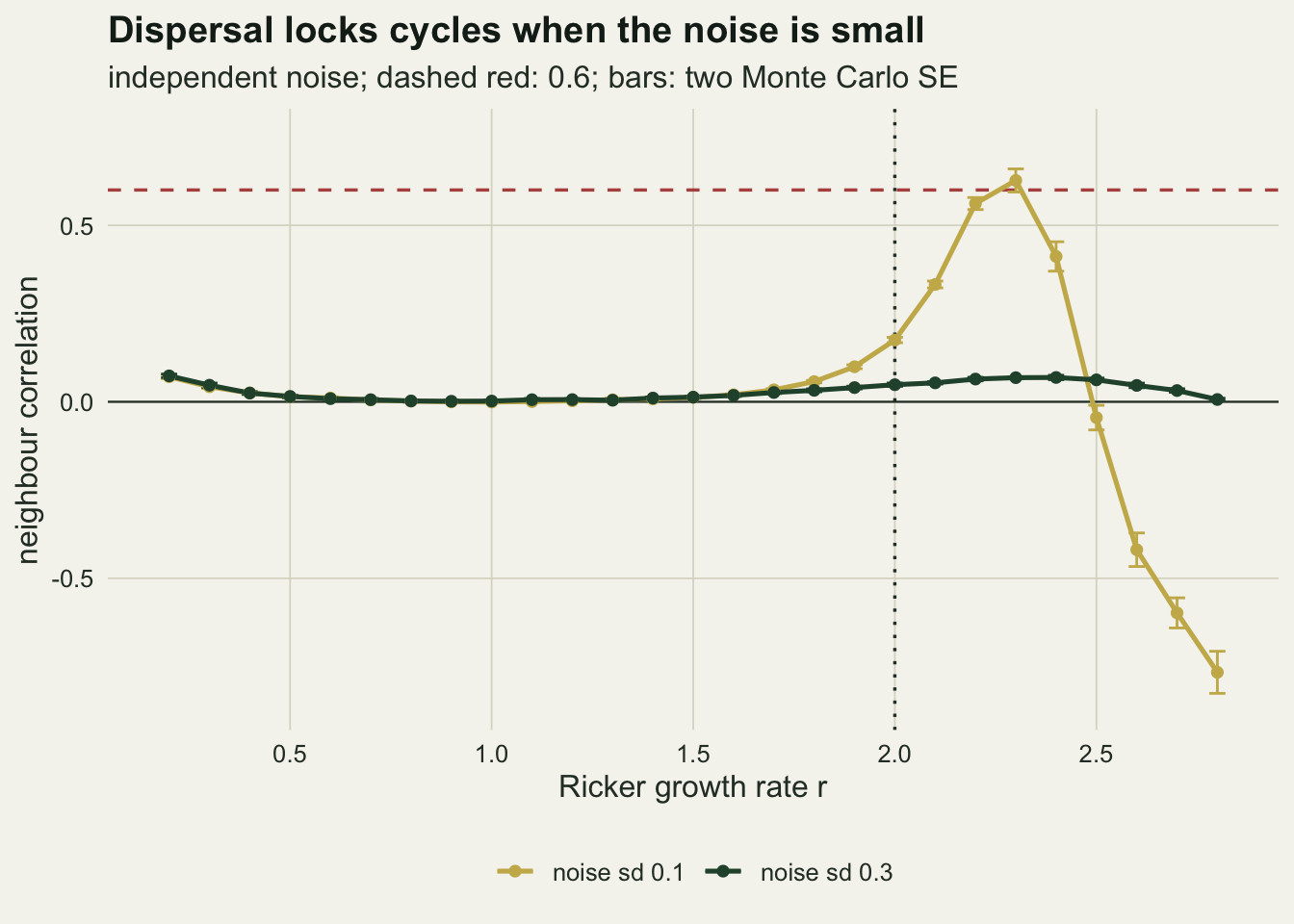
What to report
Report synchrony as what it is, a correlation of population series, and do not report it as an estimate of the environmental correlation unless the conditions of the theorem have been argued for. The two conditions that matter in practice are that the populations share their density dependence and that the dynamics are close to linear over the range the counts actually visit. The first can be checked roughly by fitting the Gompertz coefficient per population, with the caveat from the density dependence post that the estimate is biased in short series; the second by looking at whether a Ricker or Gompertz fit shows overcompensation or cycles.
Give the uncertainty of each pairwise correlation, or at least the length of the series and the autocorrelation, because the spread of a thirty year estimate is the largest source of error measured here. A mean correlation over many pairs at the same distance is far more stable than any single pair, which is why distance decay curves are usually built from all pairs in a network.
Do not attribute synchrony to the Moran effect because it decays with distance, or to dispersal because it decays quickly. A shared weather field decaying with distance and a dispersal process can produce the same profile, and in the ring above even the lag one statistics barely separate them. Nor does weak synchrony under strong density dependence rule dispersal out: that holds for stable linear dynamics, and a cycling population can be phase locked by very little movement. Independent evidence settles mechanism: measured weather correlations, marked animals, or an experiment.
Honest limits
The linear dispersal ring mixes log abundances, which is an approximation to moving individuals that holds for small deviations from equilibrium; the Ricker ring moves individuals and needs no such approximation. Its conclusion, that dispersal synchronises little under strong regulation, is a result about linear stable dynamics and is contradicted by the cycling ring, so it should not be quoted without that condition. The cycling result has its own limits. Phase locking was measured at two noise levels only, it was present at the smaller and absent at the larger, and the noise level at which it gives way was not located. The ring has sixteen estates, an even number, which lets the alternating pattern at high growth rates close on itself; an odd ring cannot alternate all the way round, and that case was not run. The timing of weather relative to movement was varied at one growth rate in the Ricker ring and exactly in the linear ring, and both rings have only nearest neighbour movement and a single dispersal rate; longer tailed dispersal would flatten the dispersal profile and move the comparison of decay rates, so the statement that dispersal synchrony was more local here belongs to this kernel and these constants, not to dispersal in general.
The Moran scenario used an exponential noise decay with a factor of 0.6 per step. That choice sets the Moran profile completely, and a different weather field would give a different curve. The fair comparison is the one made in the impostor chunk, not the visual one in the left panel: any profile can be matched.
All populations are observed without error. Observation error adds independent noise to each count series and lowers the sample correlation below the process correlation, so in real counts the equality fails even when the theorem holds for the underlying populations. The size of that attenuation depends on the ratio of observation to process variance, which this post does not vary.
Noise correlation is contemporaneous throughout. A weather effect that acts on one population in the same year and on another a year later, through a different life stage, breaks the theorem in yet another way that is not measured here. The Ricker results cover one functional form and two noise levels; other nonlinear models, and demographic stochasticity in small populations, will break the equality at different points.
References
Moran PAP 1953 Australian Journal of Zoology 1(3):291-298 (10.1071/ZO9530291)
Liebhold A, Koenig WD, Bjornstad ON 2004 Annual Review of Ecology, Evolution, and Systematics 35:467-490 (10.1146/annurev.ecolsys.34.011802.132516)
Kendall BE, Bjornstad ON, Bascompte J, Keitt TH, Fagan WF 2000 The American Naturalist 155(5):628-636 (10.1086/303350)
Grenfell BT, Wilson K, Finkenstadt BF, Coulson TN, Murray S, Albon SD, Pemberton JM, Clutton-Brock TH, Crawley MJ 1998 Nature 394(6694):674-677 (10.1038/29291)