library(ggplot2)

dgev <- function(x, mu, sigma, xi) {
  z <- (x - mu) / sigma
  if (abs(xi) < 1e-8) {
    exp(-z) * exp(-exp(-z)) / sigma
  } else {
    t <- 1 + xi * z
    d <- numeric(length(x))
    ok <- t > 0
    d[ok] <- (1 / sigma) * t[ok]^(-1 / xi - 1) * exp(-t[ok]^(-1 / xi))
    d
  }
}
qgev <- function(p, mu, sigma, xi) {
  if (abs(xi) < 1e-8) mu - sigma * log(-log(p))
  else mu - (sigma / xi) * (1 - (-log(p))^(-xi))
}
rgev <- function(n, mu, sigma, xi) qgev(runif(n), mu, sigma, xi)

# a Weibull-type GEV has a hard ceiling; a Frechet-type one does not
weibull_endpoint <- 31 - 1.6 / (-0.25)Block maxima and the GEV distribution
R
extreme value theory
statistics
ecology tutorial
Fit the generalised extreme value distribution to annual maxima in R from scratch, read the shape parameter, and see why the tail is hard to pin down.
Corrected 1 October 2026: the return level section said a long return level extrapolates past the largest value ever observed; here the fitted levels fall below that value, and the text now says that what is extrapolated is the return period, which runs beyond the length of the record.
Corrected 30 September 2026: the introduction and closing said block maxima are guaranteed to converge to the GEV; the theorem says that if rescaled maxima converge at all, the limit is a GEV, and the text now says that.
Most of the statistics on this blog is about the middle of a distribution: the mean response, the typical slope, the average abundance. But a great deal of ecology is decided at the edges. A population is not killed by an average summer; it is killed by the hottest day in a decade. A shore community is not reshaped by a typical wave; it is reshaped by the largest storm in fifty years. Gaines and Denny (1993) made this point plainly: biostatistics trains ecologists to think about central tendency, yet many of the questions that matter concern the largest, smallest, highest and lowest values a system ever sees.
Extreme value theory gives those questions a proper footing. This post covers the block maxima approach: split a long record into blocks (usually years), keep the maximum of each block, and fit the one family of distributions that rescaled block maxima can converge to. We build the likelihood by hand so nothing is hidden, and we end on the honest catch that the whole cluster returns to: the parameter that governs the tail is the hardest one to estimate, and a few decades of maxima barely constrain it.
The one distribution block maxima can converge to
Suppose you take the maximum of a large number of independent observations. As the block size grows, the (suitably rescaled) maximum can only settle down to one family of distributions, whatever the underlying data look like. This is the extremal types theorem of Fisher and Tippett (1928), later given its general form by Gnedenko (1943), and it is the extreme value analogue of the central limit theorem. The limiting family is the generalised extreme value (GEV) distribution, with distribution function
\[G(z) = \exp\left\{-\left[1 + \xi\,\frac{z-\mu}{\sigma}\right]^{-1/\xi}\right\}, \qquad 1 + \xi\,\frac{z-\mu}{\sigma} > 0,\]
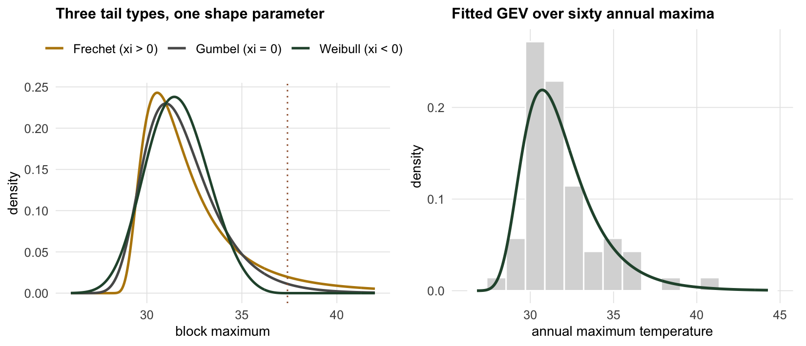
for location \(\mu\), scale \(\sigma > 0\) and shape \(\xi\). The shape parameter is the whole story. It sorts the GEV into three tail behaviours:
- \(\xi = 0\) (the Gumbel limit): a light, exponential-like tail. Maxima of Gaussian, exponential and lognormal data head here.
- \(\xi > 0\) (the Frechet limit): a heavy, polynomial tail with no upper bound. Maxima of heavy-tailed data head here.
- \(\xi < 0\) (the Weibull limit): a bounded tail with a finite upper endpoint at \(\mu - \sigma/\xi\).
Base R has no GEV functions, so we write the density, quantile and random generator ourselves. There is nothing to install.
A Weibull-type fit with \(\mu = 31\), \(\sigma = 1.6\) and \(\xi = -0.25\) places a physical ceiling on the variable at 37.4: no matter how long you wait, the block maximum cannot exceed it. That is a strong biological claim, and whether it is warranted comes down to the sign of \(\xi\), which is exactly the quantity the data struggle to resolve.
Fitting the GEV to annual maxima
Take a concrete ecological setting: the annual maximum daily temperature at a site, recorded for sixty years. High-temperature extremes drive thermal stress and mortality, so the quantity of interest is not the average summer but the hottest day each year. We simulate sixty annual maxima from a GEV with a mildly heavy tail, then recover the parameters as if we did not know them.
nll_gev <- function(par, x) {
  mu <- par[1]; sigma <- exp(par[2]); xi <- par[3]   # log-scale keeps sigma > 0
  z <- (x - mu) / sigma
  if (abs(xi) < 1e-6) {
    ll <- -log(sigma) - z - exp(-z)
  } else {
    t <- 1 + xi * z
    if (any(t <= 0)) return(1e10)
    ll <- -log(sigma) - (1 / xi + 1) * log(t) - t^(-1 / xi)
  }
  -sum(ll)
}
fit_gev <- function(x) {
  s0 <- sd(x) * sqrt(6) / pi                 # moment starts (Gumbel)
  mu0 <- mean(x) - 0.5772 * s0
  o <- optim(c(mu0, log(s0), 0.1), nll_gev, x = x,
             method = "BFGS", hessian = TRUE)
  # a second start: BFGS can stall against the support boundary
  o2 <- optim(c(mu0, log(s0), -0.1), nll_gev, x = x,
              method = "BFGS", hessian = TRUE)
  if (o2$value < o$value) o <- o2
  se <- sqrt(diag(solve(o$hessian)))
  list(mu = o$par[1], sigma = exp(o$par[2]), xi = o$par[3],
       se_mu = se[1], se_xi = se[3])
}

set.seed(4246)
mu_true <- 31.0; sigma_true <- 1.6; xi_true <- 0.13
ymax <- rgev(60, mu_true, sigma_true, xi_true)   # sixty annual maxima
fit <- fit_gev(ymax)
xi_lo <- fit$xi - 1.96 * fit$se_xi
xi_hi <- fit$xi + 1.96 * fit$se_xi
The maximum likelihood fit gives a location of 30.82 (standard error 0.24) and a scale of 1.68, against the true 31.0 and 1.6. The location is pinned down well: sixty maxima are plenty to say where the distribution sits.
The shape is another matter. The estimate is 0.060 with a standard error of 0.081, so a Wald interval runs from -0.10 to 0.22, against a true value of 0.13. Read that interval against the three tail types before reading the point estimate: an interval that spans zero leaves it open whether the tail is heavy, light or bounded, whatever sign the estimate itself carries. This is not a failing of the code; it is intrinsic. The shape parameter is estimated from the handful of largest maxima, and a few decades simply do not contain many of those.
Return levels: reading the fit as a design number
The reason to fit a GEV is rarely the density itself. It is the return level: the value expected to be exceeded once, on average, every \(m\) blocks. For annual maxima that is the \(m\)-year event. The \(m\)-year return level is the \((1 - 1/m)\) quantile of the GEV,
\[z_m = \mu - \frac{\sigma}{\xi}\left[1 - \{-\log(1 - 1/m)\}^{-\xi}\right],\]
which is just our quantile function evaluated at \(p = 1 - 1/m\).
return_level <- function(fit, m) qgev(1 - 1 / m, fit$mu, fit$sigma, fit$xi)
rl50  <- return_level(fit, 50)
rl100 <- return_level(fit, 100)
rl50_true  <- qgev(1 - 1 / 50,  mu_true, sigma_true, xi_true)
rl100_true <- qgev(1 - 1 / 100, mu_true, sigma_true, xi_true)
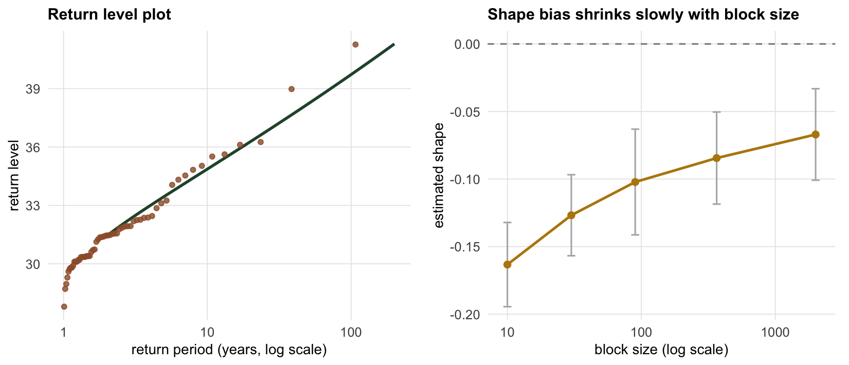
The fitted 50-year return level is 38.2 and the 100-year level is 39.7. The true values, which we happen to know, are 39.1 and 41.1. The return level for a long return period is dominated by \(\xi\). A small change in the shape, well within its standard error, moves the 100-year temperature by more than a degree. The return level inherits all of the shape parameter’s uncertainty and then some, because a long return period asks about more years than the record holds, so the fitted curve is carried beyond the length of the record. The uncertainty in that extrapolation is the subject of a later tutorial.
The block size is a bias against variance trade
The GEV is a limit as the block size grows. For a finite block it is an approximation, and the quality of the approximation depends on the underlying data. Gaussian data are the notorious case: the maximum of a Gaussian sample converges to the Gumbel form (\(\xi = 0\)), but it does so at a logarithmic rate, which is painfully slow. Fit a GEV to maxima taken over short blocks and \(\hat\xi\) is pulled well below zero, wrongly suggesting a bounded tail.
We can see the systematic bias directly by taking maxima over blocks of increasing length and looking at the average \(\hat\xi\), rather than relying on any single noisy dataset.
set.seed(202)
block_sizes <- c(10, 30, 90, 365, 2000)
bias_tab <- data.frame(block = block_sizes, xi = NA_real_, sd = NA_real_)
for (i in seq_along(block_sizes)) {
  xis <- replicate(30, {
    M <- replicate(400, max(rnorm(block_sizes[i])))
    fit_gev(M)$xi
  })
  bias_tab$xi[i] <- mean(xis)
  bias_tab$sd[i] <- sd(xis)
}
xi_small <- bias_tab$xi[bias_tab$block == 10]
xi_big   <- bias_tab$xi[bias_tab$block == 2000]
Blocks of ten give an average shape of -0.163, blocks of two thousand give -0.067, and the true limit is exactly zero. Even blocks of two thousand have not arrived. This is the bias side of the trade. The variance side is the mirror image: for a fixed length of record, longer blocks mean fewer maxima to fit, so the estimates get noisier. There is no block size that is right in general. Annual blocks are the convention because a year is a natural unit and it usually keeps the approximation acceptable, but the choice is a modelling decision, not a fact about the data.
What to take away
Block maxima give a principled way to model the largest value a system produces in each period, and the GEV is the only limiting distribution they can follow. Fitting it by hand is a short piece of code. The honest parts are the ones worth remembering. The location is easy; the shape parameter, which decides whether the tail is heavy, light or bounded, and which drives every long return level, is estimated from only the largest few maxima and carries wide uncertainty. The block size trades bias for variance with no objective optimum. And a long return level is an extrapolation beyond the length of the record, so it is only as trustworthy as the shape parameter that steers it. The next tutorial keeps every value above a high threshold instead of one per block, which uses the data more efficiently and shifts the difficulty from the block size to the threshold.
References
Fisher, R.A. and Tippett, L.H.C. 1928. Proceedings of the Cambridge Philosophical Society 24(2):180-190 (10.1017/S0305004100015681).
Gnedenko, B. 1943. Annals of Mathematics 44(3):423-453 (10.2307/1968974).
Gaines, S.D. and Denny, M.W. 1993. Ecology 74(6):1677-1692 (10.2307/1939926).
Katz, R.W., Brush, G.S. and Parlange, M.B. 2005. Ecology 86(5):1124-1134 (10.1890/04-0606).
Coles, S. 2001. An Introduction to Statistical Modeling of Extreme Values. Springer (ISBN 978-1-85233-459-8).