library(ggplot2)

te_paper  <- "#f5f4ee"
te_ink    <- "#16241d"
te_body   <- "#2c3a31"
te_forest <- "#275139"
te_rust   <- "#b5534e"
te_gold   <- "#c9b458"
te_line   <- "#dad9ca"

theme_datasheet <- function() {
  theme_minimal(base_size = 12) +
    theme(plot.background  = element_rect(fill = te_paper, colour = NA),
          panel.background = element_rect(fill = te_paper, colour = NA),
          panel.grid.major = element_line(colour = te_line, linewidth = 0.3),
          panel.grid.minor = element_blank(),
          text             = element_text(colour = te_body),
          plot.title       = element_text(colour = te_ink, face = "bold"),
          plot.subtitle    = element_text(colour = te_body),
          axis.text        = element_text(colour = te_body),
          strip.text       = element_text(colour = te_ink))
}Richness from stacked SDMs: sum the probabilities
R
species distribution models
species richness
simulation
ecology tutorial
Stacking thresholded species distribution models over-predicts richness and stretches its contrast. Summing probabilities does not; with an interval, in R.
A regional conservation plan needs a map of plant species richness on a grid of sixty by sixty cells. There is a survey of four hundred cells with presence and absence for sixty species, and two climate and habitat layers that cover the whole grid. The usual route is to fit one species distribution model per species, project each over the grid, turn each projection into a presence map with a threshold, often the one that maximises the true skill statistic (TSS), and add the sixty maps together. A second route skips the models: draw a polygon around each species’ records, treat everything inside as occupied, and add the polygons. Both routes produce a richness map that looks plausible, and both are wrong in ways that can be measured.
This post measures them against the alternative that needs no threshold at all: add up the fitted probabilities. If each model gives the probability that its species is present in a cell, the expected number of species in that cell is the sum of those probabilities, by nothing more than linearity of expectation. Calabrese and colleagues (2014) set out why stacking thresholded predictions biases richness and why summed probabilities do not, and they gave the Poisson-binomial distribution of richness that follows from summing, under an explicit assumption that species are independent. The simulation below demonstrates their point on a known truth and then measures three things around it: how the binary stack distorts the contrast between rich and poor cells, how often the Poisson-binomial interval covers the realised count and what happens to it when species share a driver, and how the answer depends on the grain at which richness is asked for.
The per-species reason for the over-prediction is already on this site. Choosing a decision threshold from costs shows that for a calibrated model the max-TSS cut sits where the threshold equals the prevalence, so a species with a prevalence of a few per cent is declared present wherever its probability exceeds a few per cent. That post is about one species and one decision; here the question is what happens when sixty such decisions are added. Joint species distribution models in R compares a stacked fit with a joint one and shows that the coefficients are identical, with the joint model’s gain lying in the residual covariance and in conditional prediction; that residual covariance is exactly what the independence assumption behind the richness interval below leaves out. Mapping species richness in R with sf builds a richness map by counting raw records in each cell, with no model, and range size distributions measures extent of occurrence, the convex hull of one species’ records, for single species rather than stacked. The mid-domain effect as a null for richness notes among its limits that real range extents are interpolated between records; the hull stack below is that interpolation drawn in two dimensions and added up. Nothing here re-teaches those.
Sixty species on a grid with a known truth
The grid has 60 by 60 cells. The first covariate is a broad north to south gradient with smooth wiggles, standing in for temperature; the second is a smooth random field, standing in for a habitat variable such as soil moisture. Two constructions are run. In the niche construction every species has a Gaussian response on the logit scale in both covariates, with its own optimum, width and peak. In the monotone construction the habitat response is a straight rise instead, so every species prefers the same end of the habitat axis and differs only in its temperature niche. Each species is then present or absent in each cell by an independent draw from its probability.
Four hundred cells are surveyed at random. For each species with at least five presences in the survey a logistic regression with linear and squared terms in both covariates is fitted to the survey cells and projected over the grid; that model family contains the true niche response and nests the monotone one. A species with fewer than five presences is not modelled, as is common practice, and its summed-probability contribution is its survey prevalence everywhere. Four stacks are built from the fitted probabilities: the plain sum, and three binary stacks with a threshold per species, at the max-TSS cut chosen on the survey cells, at the survey prevalence, and at 0.5. The TSS is sensitivity plus specificity minus one (Allouche and colleagues 2006). A fifth stack applies the max-TSS rule to the true probabilities, chosen on the full grid, as an oracle with no estimation error. The range-map stack uses, for each species, the convex hull of its survey presence cells. Every stack is compared with the realised richness on every cell that was not surveyed.
side     <- 60
n_cell   <- side^2
n_sp     <- 60
n_surv   <- 400
min_pres <- 5
grain_set <- c(1, 2, 3, 5, 10, 15, 20, 30)
gx <- rep(seq_len(side), times = side)
gy <- rep(seq_len(side), each = side)

smooth_field <- function(k = 6) {
  f <- 0
  for (i in seq_len(k)) {
    a  <- runif(2, 0.05, 0.25)
    ph <- runif(2, 0, 2 * pi)
    f  <- f + sin(a[1] * gx + ph[1]) * cos(a[2] * gy + ph[2])
  }
  as.numeric(scale(f))
}

in_hull <- function(ids) {
  inside <- rep(FALSE, n_cell)
  if (length(ids) < 3) { inside[ids] <- TRUE; return(inside) }
  pts  <- cbind(gx[ids], gy[ids])
  poly <- pts[chull(pts), , drop = FALSE]
  m <- nrow(poly)
  pos <- rep(TRUE, n_cell); neg <- rep(TRUE, n_cell)
  for (k in seq_len(m)) {
    a  <- poly[k, ]
    b  <- poly[if (k == m) 1 else k + 1, ]
    cr <- (b[1] - a[1]) * (gy - a[2]) - (b[2] - a[2]) * (gx - a[1])
    pos <- pos & cr >= -1e-9
    neg <- neg & cr <= 1e-9
  }
  inside <- pos | neg
  inside[ids] <- TRUE
  inside
}

max_tss_cut <- function(p_fit, y) {
  o   <- order(p_fit, decreasing = TRUE)
  ps  <- p_fit[o]
  ys  <- y[o]
  tss <- cumsum(ys) / sum(ys) + (sum(1 - ys) - cumsum(1 - ys)) / sum(1 - ys) - 1
  tss[c(ps[-1] == ps[-length(ps)], FALSE)] <- -Inf
  ps[which.max(tss)]
}

pb_pmf <- function(p_mat) {
  pmf <- matrix(0, nrow(p_mat), ncol(p_mat) + 1)
  pmf[, 1] <- 1
  for (j in seq_len(ncol(p_mat))) {
    pj  <- p_mat[, j]
    pmf <- pmf * (1 - pj) + cbind(0, pmf[, -ncol(pmf), drop = FALSE]) * pj
  }
  pmf
}

pb_interval <- function(p_mat, level = 0.90) {
  cdf <- t(apply(pb_pmf(p_mat), 1, cumsum))
  a <- (1 - level) / 2
  cbind(lo = rowSums(cdf < a), hi = rowSums(cdf < 1 - a))
}
The function below builds one world, fits the models and returns the summaries used in the rest of the post. The shared argument adds an unmeasured site effect, common to all species, that is switched off until the section on intervals.
one_world <- function(kind = "niche", shared = 0, grains = TRUE, keep = FALSE) {
  x1 <- as.numeric(scale(gy + 8 * smooth_field()))
  x2 <- smooth_field()
  site_eff <- shared * as.numeric(scale(rnorm(n_cell)))
  u1 <- runif(n_sp, -2, 2);    u2 <- runif(n_sp, -1.5, 1.5)
  w1 <- runif(n_sp, 0.4, 1.2); w2 <- runif(n_sp, 0.5, 1.5)
  h  <- runif(n_sp, -3, 2);    bh <- runif(n_sp, 0.5, 1.5)
  eta <- sapply(seq_len(n_sp), function(j) h[j] - (x1 - u1[j])^2 / (2 * w1[j]^2) +
    if (kind == "monotone") bh[j] * x2 else -(x2 - u2[j])^2 / (2 * w2[j]^2))
  p_true <- plogis(eta + site_eff)
  occ    <- matrix(rbinom(n_cell * n_sp, 1, p_true), n_cell)
  surv   <- sample.int(n_cell, n_surv)
  test   <- setdiff(seq_len(n_cell), surv)

  p_hat  <- matrix(0, n_cell, n_sp)
  b_tss  <- matrix(FALSE, n_cell, n_sp)
  b_half <- b_tss; b_prev <- b_tss; b_orac <- b_tss; hull <- b_tss
  fitted <- logical(n_sp); prev <- numeric(n_sp)
  newd <- data.frame(a = x1, b = x2)
  for (j in seq_len(n_sp)) {
    y <- occ[surv, j]
    prev[j]     <- mean(y)
    hull[, j]   <- in_hull(surv[y == 1])
    b_orac[, j] <- p_true[, j] >= max_tss_cut(p_true[, j], occ[, j])
    if (sum(y) < min_pres) { p_hat[, j] <- prev[j]; next }
    fitted[j] <- TRUE
    fit <- suppressWarnings(glm(y ~ a + I(a^2) + b + I(b^2), family = binomial,
                                data = data.frame(y, a = x1[surv], b = x2[surv])))
    p_hat[, j]  <- predict(fit, newd, type = "response")
    b_tss[, j]  <- p_hat[, j] >= max_tss_cut(p_hat[surv, j], y)
    b_half[, j] <- p_hat[, j] >= 0.5
    b_prev[, j] <- p_hat[, j] >= prev[j]
  }
  s_true <- rowSums(occ)
  s_exp  <- rowSums(p_true)
  est <- cbind(sum_p = rowSums(p_hat), max_tss = rowSums(b_tss), cut_half = rowSums(b_half),
               cut_prev = rowSums(b_prev), oracle = rowSums(b_orac), hull = rowSums(hull))
  tt <- test
  sp_excess <- colMeans(b_tss[tt, ]) - colMeans(p_hat[tt, ])
  stopifnot(abs(mean(est[tt, "max_tss"]) - mean(est[tt, "sum_p"]) - sum(sp_excess)) < 1e-9)
  poor    <- s_exp[tt] <= quantile(s_exp[tt], 0.25)
  iv_hat  <- pb_interval(p_hat[tt, ])
  iv_true <- pb_interval(p_true[tt, ])
  st <- c(n_fit = sum(fitted), unfit_share = sum(occ[tt, !fitted]) / sum(occ[tt, ]),
          mean_s = mean(s_true[tt]),
          setNames(colMeans(est[tt, ]) / mean(s_true[tt]), paste0("ratio_", colnames(est))),
          setNames(apply(est[tt, ], 2, function(v) unname(coef(lm(v ~ s_exp[tt]))[2])),
                   paste0("calib_", colnames(est))),
          setNames(apply(est[tt, ], 2, function(v) cor(v, s_true[tt])),
                   paste0("cor_", colnames(est))),
          setNames(colMeans(est[tt[poor], ]) / mean(s_true[tt[poor]]),
                   paste0("poor_", colnames(est))),
          excess_sum = sum(sp_excess),
          cov_hat   = mean(s_true[tt] >= iv_hat[, "lo"] & s_true[tt] <= iv_hat[, "hi"]),
          cov_true  = mean(s_true[tt] >= iv_true[, "lo"] & s_true[tt] <= iv_true[, "hi"]),
          var_ratio = mean((s_true[tt] - est[tt, "sum_p"])^2) /
                      mean(rowSums(p_hat[tt, ] * (1 - p_hat[tt, ]))),
          var_ratio_true = mean((s_true[tt] - s_exp[tt])^2) /
                           mean(rowSums(p_true[tt, ] * (1 - p_true[tt, ]))),
          cor_exp = cor(s_exp[tt], s_true[tt]))
  stopifnot(abs(st["ratio_max_tss"] - st["ratio_sum_p"] - st["excess_sum"] / st["mean_s"]) < 1e-9)
  out <- list(stats = st,
              species = data.frame(kind, prev = prev[fitted], excess = sp_excess[fitted]))
  if (grains) {
    out$grain <- do.call(rbind, lapply(grain_set, function(g) {
      blk   <- (ceiling(gx / g) - 1) * (side / g) + ceiling(gy / g)
      s_blk <- rowSums(rowsum(occ, blk) > 0)
      data.frame(kind, g,
                 hull    = mean(rowSums(rowsum(hull + 0, blk) > 0)) / mean(s_blk),
                 max_tss = mean(rowSums(rowsum(b_tss + 0, blk) > 0)) / mean(s_blk),
                 prob    = mean(rowSums(1 - exp(rowsum(log1p(-p_hat), blk)))) / mean(s_blk))
    }))
    stopifnot(abs(out$grain$hull[1] - sum(hull) / sum(occ)) < 1e-9)
  }
  if (keep) out$cells <- data.frame(kind, gx, gy, test = seq_len(n_cell) %in% test,
                                    s_true, s_exp, est)
  out
}
Summed probabilities against binary stacks
Twenty worlds of each construction are drawn, each with new covariate fields, new species and a new survey. Every summary below is a mean over worlds with its Monte Carlo standard error.
n_world <- 20
set.seed(43101)
runs <- list()
for (k in c("niche", "monotone")) for (r in seq_len(n_world))
  runs[[length(runs) + 1]] <- one_world(k, keep = r == 1)

stat_tab <- data.frame(kind = rep(c("niche", "monotone"), each = n_world),
                       do.call(rbind, lapply(runs, `[[`, "stats")))
stat_tab$excess_rel <- stat_tab$excess_sum / stat_tab$mean_s
mean_tab <- aggregate(. ~ kind, stat_tab, mean)
se_tab   <- aggregate(. ~ kind, stat_tab, function(v) sd(v) / sqrt(length(v)))
mv  <- function(k, v) mean_tab[mean_tab$kind == k, v]
msd <- function(k, v) se_tab[se_tab$kind == k, v]
rng <- function(k, v) range(stat_tab[stat_tab$kind == k, v])
stopifnot(min(stat_tab$ratio_max_tss) > 1, min(stat_tab$ratio_cut_half) < 1)
On average 56.9 of the 60 species are modelled in the niche worlds and 59.7 in the monotone ones; the unmodelled species account for 0.34 and 0.03 per cent of the realised occurrences on the unsurveyed cells. Mean realised richness per cell is 9.3 species in the niche worlds and 14.5 in the monotone ones.
The summed probabilities give a mean richness of 1.000 times the realised mean in the niche worlds and 0.996 times in the monotone ones (standard errors 0.002 and 0.002). The max-TSS stack gives 2.35 times (standard error 0.06, single worlds from 1.85 to 3.02) and 1.62 times (standard error 0.04, single worlds from 1.39 to 2.11). Cutting at the survey prevalence gives 2.42 and 1.66, close to the max-TSS stack, as the threshold post would predict. The fixed cut at 0.5 goes the other way, 0.71 and 0.83, because a species whose fitted probability never reaches one half is never counted. The record hulls give 3.44 and 2.67.
The over-prediction is not an estimation problem. The oracle stack, which applies the max-TSS rule to the true probabilities, gives 2.57 and 1.68. How large the factor is depends on the construction, through the mix of species prevalences and the shape of each species’ probability surface, and a different species pool would give a different factor; the factor is arithmetic of the probabilities and the cuts, derived in the next section. There is no single correction factor to apply.
ex_niche <- runs[[1]]$cells
map_long <- rbind(
  data.frame(ex_niche[, c("gx", "gy")], what = "realised richness", s = ex_niche$s_true),
  data.frame(ex_niche[, c("gx", "gy")], what = "summed probabilities", s = ex_niche$sum_p),
  data.frame(ex_niche[, c("gx", "gy")], what = "max-TSS stack", s = ex_niche$max_tss),
  data.frame(ex_niche[, c("gx", "gy")], what = "record hulls", s = ex_niche$hull))
map_long$what <- factor(map_long$what, c("realised richness", "summed probabilities",
                                         "max-TSS stack", "record hulls"))

ggplot(map_long, aes(gx, gy, fill = s)) +
  geom_raster() +
  facet_wrap(~ what, nrow = 2) +
  scale_fill_gradientn(colours = c(te_paper, te_gold, te_forest, te_ink), name = "species") +
  coord_equal(expand = FALSE) +
  labs(x = NULL, y = NULL, title = "Four maps of the same richness") +
  theme_datasheet() +
  theme(axis.text = element_blank(), panel.grid.major = element_blank())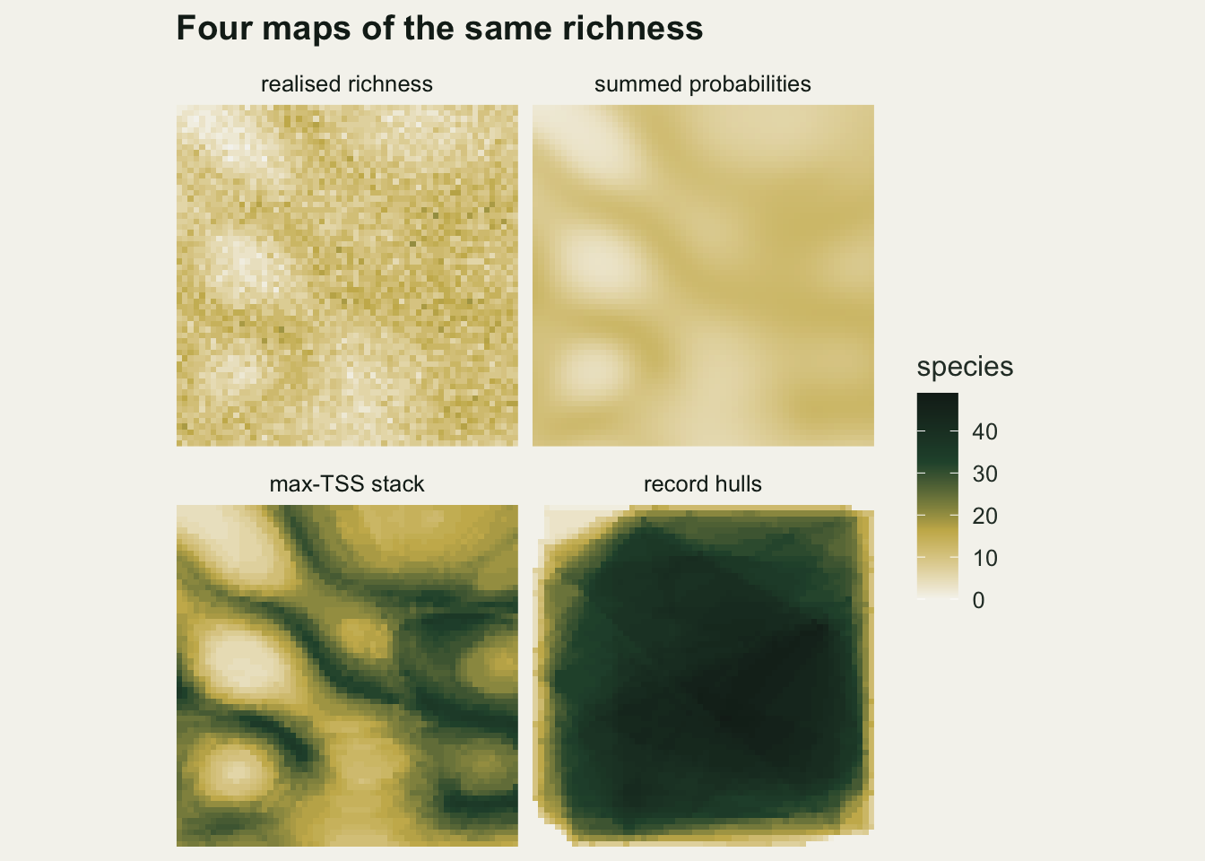
The mean excess is a sum over species
The size of the mean excess needs no simulation to explain. Over the unsurveyed cells, the mean of a binary stack is the sum over species of the share of cells in which each species is declared present, and the mean of the summed probabilities is the sum over species of each species’ mean probability. The difference between the two is therefore
mean excess = sum over species of (share of cells above the species’ cut - mean fitted probability of the species),
an identity, checked to machine precision inside one_world() by the stopifnot() line. Since the summed probabilities match the realised mean, this sum is the whole bias of the binary stack in the mean. With the cut near the prevalence, where max-TSS puts it, each term is the share of cells in which a species’ probability exceeds its own average, minus that average; for a rare species whose probability is near zero over most of the grid and high in a small area, the share above the average is several times the average. The chunk below collects the terms over all worlds.
sp_all <- do.call(rbind, lapply(runs, `[[`, "species"))
sp_all$band <- cut(sp_all$prev, c(0, 0.05, 0.2, 1), include.lowest = TRUE,
                   labels = c("rare", "middling", "common"))
band_tab <- aggregate(excess ~ kind + band, sp_all, mean)
band_n   <- aggregate(excess ~ kind + band, sp_all, length)
bv <- function(k, b) band_tab$excess[band_tab$kind == k & band_tab$band == b]
band_pw  <- function(k, b) band_n$excess[band_n$kind == k & band_n$band == b] / n_world
excess_ratio <- mv("niche", "excess_sum") / mv("monotone", "excess_sum")
mean_s_ratio <- mv("monotone", "mean_s") / mv("niche", "mean_s")
stopifnot(mean_s_ratio > excess_ratio)
neg_common <- tapply(sp_all$excess[sp_all$band == "common"] < 0,
                     sp_all$kind[sp_all$band == "common"], mean)
sp_all$kind <- factor(sp_all$kind, c("niche", "monotone"))
The mean excess is 12.3 species per cell in the niche worlds and 8.7 in the monotone ones. A modelled species with a survey prevalence of at most five per cent adds on average 0.27 of a species to every cell in the niche worlds and 0.22 in the monotone ones; one between five and twenty per cent adds 0.25 and 0.20; one above twenty per cent adds 0.13 and 0.08. Each rare or middling species contributes a similar amount, so the excess grows with the number of such species in the pool. The niche worlds hold 16.4 rare modelled species per world against 7.3 in the monotone ones, with similar numbers of middling species (22.9 and 23.8) and fewer common ones (17.6 against 28.6), so their excess is larger. That is one part of why the factor of the previous section differs. The factor of each world is exactly the ratio of its summed probabilities to its realised mean (on average the 1.000 and 0.996 above) plus its excess divided by its mean realised richness; averaged over worlds the second term is 1.35 in the niche worlds and 0.62 in the monotone ones, and one_world() checks the identity with a stopifnot(). The niche excess is 1.42 times the monotone one, but the monotone mean richness is 1.55 times the niche one: the larger denominator lowers the monotone factor by a little more than the smaller excess does. Among the common species the term is negative for 9 per cent in the niche worlds and 19 per cent in the monotone ones: their max-TSS cut lies above their mean probability, and the share of cells in which they are declared present is smaller than their mean probability.
ggplot(sp_all, aes(prev, excess)) +
  geom_hline(yintercept = 0, colour = te_body, linewidth = 0.5) +
  geom_point(colour = te_forest, alpha = 0.35, size = 1.3) +
  facet_wrap(~ kind) +
  scale_x_log10() +
  labs(x = "survey prevalence of the species (log scale)",
       y = "share above cut minus mean probability",
       title = "Rare and middling species carry the excess") +
  theme_datasheet()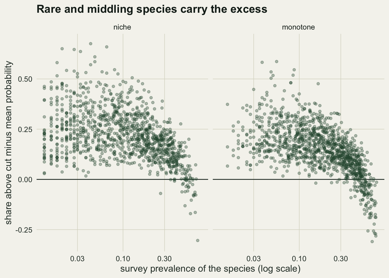
The binary stack stretches the contrast
A richness map is used for its contrasts more than for its mean: which cells are richest, how much richer than the rest. The calibration slope measures that. Regressing each estimate on the expected richness, the sum of the true probabilities, over the unsurveyed cells gives a slope of one for an estimate that keeps the contrast, above one for an estimate that exaggerates it.
calib_tab <- data.frame(stack = c("summed probabilities", "max-TSS", "prevalence cut", "cut at 0.5",
                                  "oracle max-TSS", "record hulls"),
                        niche = unlist(mean_tab[mean_tab$kind == "niche",
                          c("calib_sum_p", "calib_max_tss", "calib_cut_prev", "calib_cut_half",
                            "calib_oracle", "calib_hull")]),
                        monotone = unlist(mean_tab[mean_tab$kind == "monotone",
                          c("calib_sum_p", "calib_max_tss", "calib_cut_prev", "calib_cut_half",
                            "calib_oracle", "calib_hull")]))
print(format(calib_tab, digits = 3), row.names = FALSE)
stack niche monotone
summed probabilities 0.991 1.002
max-TSS 2.947 1.968
prevalence cut 3.037 2.017
cut at 0.5 0.850 1.170
oracle max-TSS 3.122 2.068
record hulls 1.288 0.531stopifnot(mv("niche", "poor_max_tss") < mv("niche", "ratio_max_tss"))The summed probabilities have a calibration slope of 0.99 in the niche worlds and 1.00 in the monotone ones. The max-TSS stack has 2.95 (single worlds 2.00 to 3.54) and 1.97 (1.78 to 2.19): averaged over the grid, a cell with one more expected species gains two to three species on the binary map. The reason is the same arithmetic cell by cell. In a rich cell many species have probabilities above their own low cuts and each is counted as a whole species; in a poor cell few do. The relation is not a straight line, most clearly in the monotone world of the figure below, where it is shallow among the poorest cells, steepest in the middle and shallower again among the richest; the slope is a linear summary of that curve. The oracle has 3.12 and 2.07, so this too survives perfect estimation. The record hulls have 1.29 and 0.53, but their correlation with realised richness is only 0.19 and 0.25, so their slope says little; the summed probabilities reach 0.73 and 0.94, and the max-TSS stack 0.68 and 0.90. The correlations are lower in the niche worlds for every stack, and the ceiling shows why: even the expected richness itself, the sum of the true probabilities, correlates with realised richness at only 0.74 there, against 0.94 in the monotone worlds. Realised richness in the niche worlds scatters more around its expectation, relative to how much the expectation varies across the grid.
Where on the map the inflation is largest depends on the construction. In the poorest quarter of cells, by expected richness, the max-TSS stack gives 2.07 times the realised richness in the niche worlds, a little below its overall factor there, but 0.97 times in the monotone worlds (standard error 0.05), no inflation at all: the poor cells lie at the end of the habitat axis that every species avoids, and few species pass their cuts there. A claim that species-poor cells are the most inflated would be wrong in both constructions: in the niche worlds the poorest quarter is inflated less than the unsurveyed grid as a whole, and in the monotone worlds not at all.
ex_all <- rbind(runs[[1]]$cells, runs[[n_world + 1]]$cells)
ex_all <- ex_all[ex_all$test, ]
sc_long <- rbind(
  data.frame(kind = ex_all$kind, s_exp = ex_all$s_exp, stack = "summed probabilities", s = ex_all$sum_p),
  data.frame(kind = ex_all$kind, s_exp = ex_all$s_exp, stack = "max-TSS stack", s = ex_all$max_tss),
  data.frame(kind = ex_all$kind, s_exp = ex_all$s_exp, stack = "cut at 0.5", s = ex_all$cut_half))
sc_long$stack <- factor(sc_long$stack, c("summed probabilities", "max-TSS stack", "cut at 0.5"))
sc_long$kind  <- factor(sc_long$kind, c("niche", "monotone"))

ggplot(sc_long, aes(s_exp, s)) +
  geom_abline(slope = 1, intercept = 0, linetype = "dashed", colour = te_body, linewidth = 0.5) +
  geom_point(aes(colour = stack), alpha = 0.25, size = 0.7, show.legend = FALSE) +
  facet_grid(kind ~ stack) +
  scale_colour_manual(values = c(te_forest, te_rust, te_gold)) +
  labs(x = "expected richness (sum of true probabilities)", y = "estimated richness",
       title = "Summing keeps the contrast; the binary stack stretches it") +
  theme_datasheet()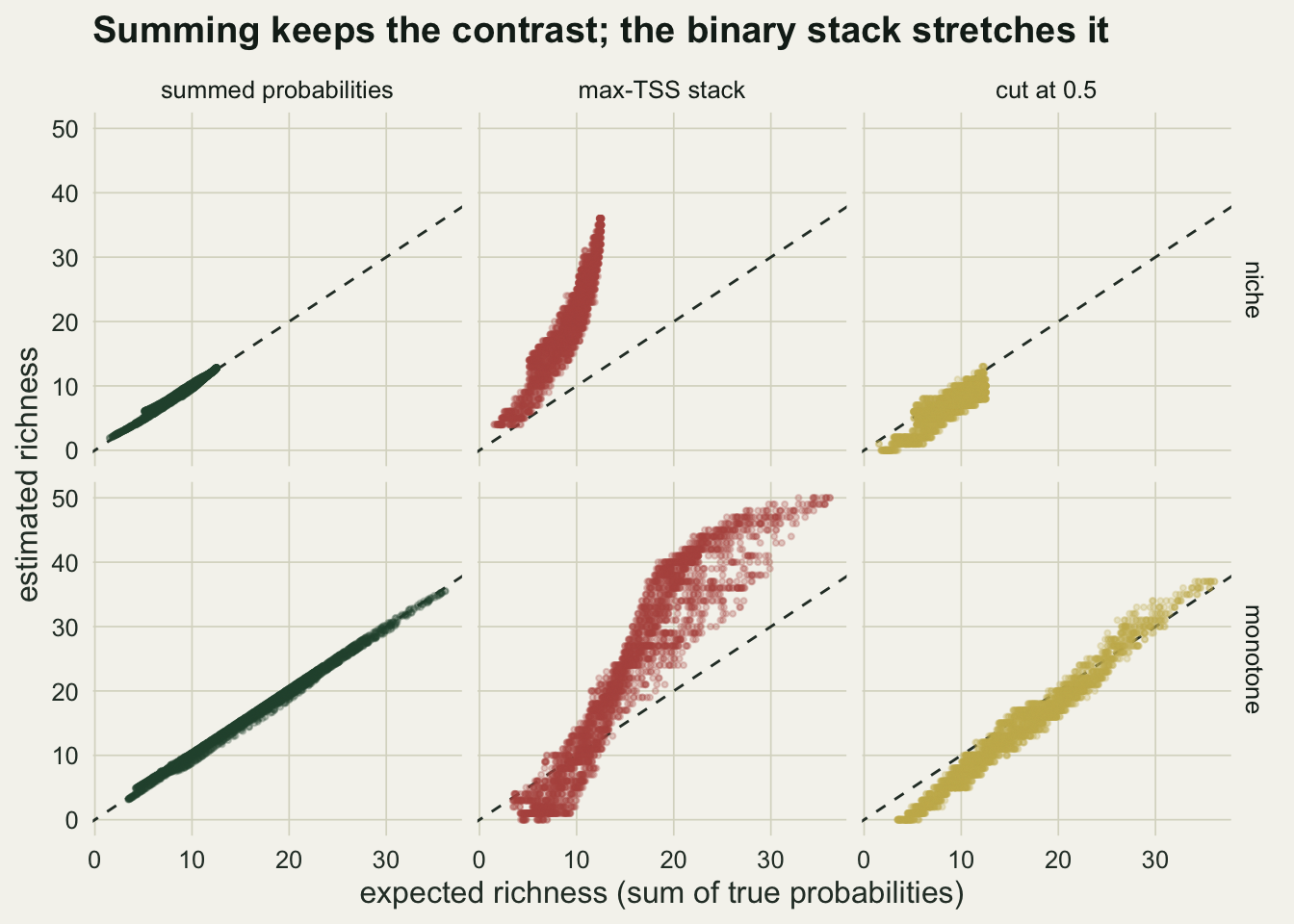
An interval for the richness of a cell
The summed probabilities give the expected richness, and a map user will want to know how far the realised count can stray from it. If species occur independently given the probabilities, the number present in a cell is a sum of independent Bernoulli variables with different probabilities, a Poisson-binomial variable (Calabrese and colleagues 2014 give this distribution for stacked models, with variance equal to the sum of p(1 - p) over species, and state the independence assumption). Its distribution is exact by convolving the species one at a time, which pb_pmf() does for all cells at once; the equal-tailed 90 per cent interval takes the smallest counts at which the cumulative distribution reaches 0.05 and 0.95. The chunk checks the convolution against the binomial for equal probabilities, and against a direct sum over all outcomes for three species.
p_eq <- matrix(rep(0.3, 10), 1)
stopifnot(max(abs(pb_pmf(p_eq) - dbinom(0:10, 10, 0.3))) < 1e-12)
p_three <- c(0.1, 0.5, 0.8)
outcomes <- as.matrix(expand.grid(0:1, 0:1, 0:1))
brute <- sapply(0:3, function(s) sum(apply(outcomes[rowSums(outcomes) == s, , drop = FALSE], 1,
  function(z) prod(ifelse(z == 1, p_three, 1 - p_three)))))
stopifnot(max(abs(pb_pmf(matrix(p_three, 1)) - brute)) < 1e-12)
stopifnot(min(stat_tab$cov_true) >= 0.90)
Because the count is an integer, an equal-tailed interval cannot hit 90 per cent exactly and errs on the wide side: with the true probabilities it covers the realised richness in 0.938 of unsurveyed cells in the niche worlds and 0.933 in the monotone ones. With the fitted probabilities it covers 0.933 and 0.928 (standard errors 0.001 and 0.001). The mean squared gap between realised richness and the summed probabilities is 1.03 and 1.04 times the mean Poisson-binomial variance. With the true probabilities in both places the same ratio is 1.000 and 1.005, so the small surplus is the estimation error of the fitted models.
The independence behind the interval is an assumption about the world, not about the models. The next chunk adds an unmeasured site effect to the logit of every species in a cell, with a standard deviation of 0.5 or 1 and independent between cells: a local condition, a disturbance or a wet hollow, that raises or lowers all species together and appears in no covariate. Ten niche worlds are run at each level.
n_shared   <- 10
shared_set <- c(0.5, 1)
set.seed(43102)
sh_runs <- do.call(rbind, lapply(shared_set, function(s) do.call(rbind, lapply(seq_len(n_shared),
  function(r) c(shared = s, one_world("niche", shared = s, grains = FALSE)$stats)))))
sh_runs <- data.frame(sh_runs)
sh_mean <- aggregate(. ~ shared, sh_runs, mean)
sh_se   <- aggregate(. ~ shared, sh_runs, function(v) sd(v) / sqrt(length(v)))
sv  <- function(s, v) sh_mean[sh_mean$shared == s, v]
sse <- function(s, v) sh_se[sh_se$shared == s, v]
The summed probabilities still get the mean right, 1.002 and 1.014 times the realised mean at the two levels (standard errors 0.005 and 0.009). The interval does not survive. Its coverage falls to 0.786 and 0.568 (standard errors 0.006 and 0.007), and the realised scatter around the summed probabilities is 2.3 and 5.7 times the Poisson-binomial variance. The species are still independent once the site effect is known: the interval built from the true probabilities, which include it, covers 0.938 and 0.937. The failure is that each fitted model averages over the site effect, and the average probabilities carry an independence that holds only given the effect. Shared residual variation of this kind is what the residual correlation of a joint model describes, and checking a joint species distribution model covers what that matrix can and cannot be trusted to show; no joint model is fitted here.
niche_rows <- stat_tab[stat_tab$kind == "niche", ]
cov_df <- rbind(
  data.frame(shared = 0, source = c("fitted probabilities", "true probabilities"),
             cov = c(mean(niche_rows$cov_hat), mean(niche_rows$cov_true)),
             se = c(sd(niche_rows$cov_hat), sd(niche_rows$cov_true)) / sqrt(n_world)),
  data.frame(shared = rep(shared_set, 2),
             source = rep(c("fitted probabilities", "true probabilities"), each = 2),
             cov = c(sv(0.5, "cov_hat"), sv(1, "cov_hat"), sv(0.5, "cov_true"), sv(1, "cov_true")),
             se = c(sse(0.5, "cov_hat"), sse(1, "cov_hat"), sse(0.5, "cov_true"), sse(1, "cov_true"))))

ggplot(cov_df, aes(shared, cov, colour = source)) +
  geom_hline(yintercept = 0.90, linetype = "dashed", colour = te_body, linewidth = 0.5) +
  geom_line(linewidth = 0.9) +
  geom_errorbar(aes(ymin = cov - 2 * se, ymax = cov + 2 * se), width = 0.03, linewidth = 0.6) +
  geom_point(size = 2.4) +
  scale_colour_manual(values = c(te_rust, te_forest), name = NULL) +
  scale_x_continuous(breaks = c(0, shared_set)) +
  scale_y_continuous(limits = c(0.5, 1)) +
  labs(x = "SD of the shared site effect on the logit scale", y = "coverage of the 90% interval",
       title = "A shared driver breaks the independence interval") +
  theme_datasheet() +
  theme(legend.position = "bottom")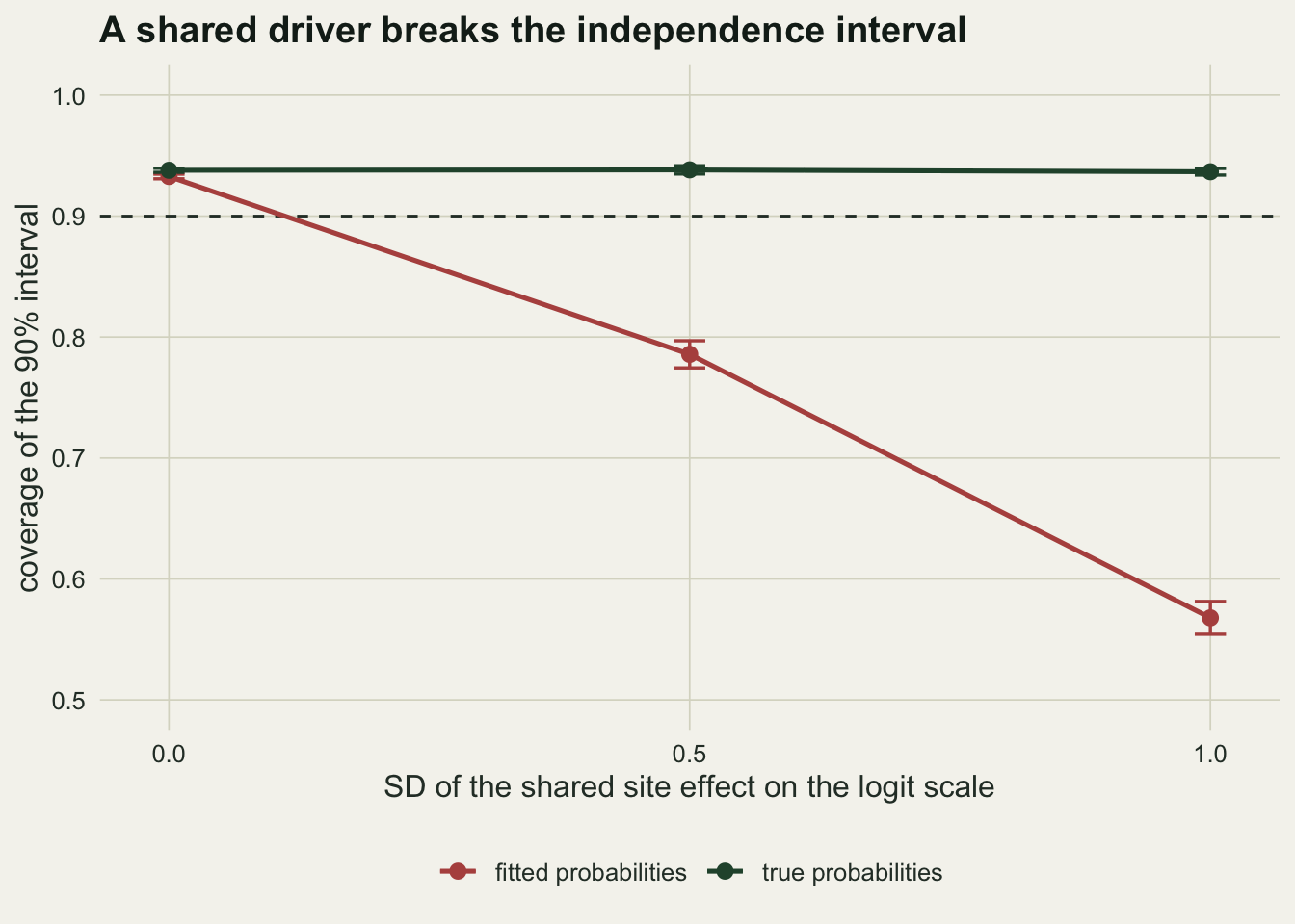
Range maps and the grain of the question
A hull around a species’ records claims the species in every cell inside it, but the species occupies only some of them. At the grain of a single cell the ratio of the hull stack to realised richness, over the whole grid, is therefore the total hull area divided by the total number of occupied cells, both summed over species; one_world() checks that identity. Its excess is arithmetic and says only that a hull is not an occupancy map, which is the point Hurlbert and Jetz (2007) made with bird range maps: they overstate occurrence at fine grain and describe richness patterns only at coarse grain. The question that is not arithmetic is how quickly each stack approaches the truth as cells are merged into blocks.
At a block of several cells, richness is the number of species present in at least one of its cells, and the summed probabilities of single cells are no longer the right quantity. If a species occurs independently across cells with the fitted probabilities, the probability that it is present somewhere in a block is one minus the product of its absence probabilities, 1 - prod(1 - p), and the expected block richness is the sum of that over species. This assumes that, given the probabilities, a species’ occurrences in neighbouring cells are independent, which is how they are drawn here, so the result below for 1 - prod(1 - p) is built in apart from the error of the fitted models and of the unmodelled species. Occurrences clumped beyond what the covariates explain would make it over-predict block richness. For the binary stack a species counts in a block when any of its cells is declared present; for the hulls, when the hull touches the block. The chunk collects the three ratios to the realised block richness, computed over the whole grid.
grain_all <- do.call(rbind, lapply(runs, `[[`, "grain"))
grain_tab <- aggregate(cbind(hull, max_tss, prob) ~ kind + g, grain_all, mean)
gv <- function(k, g, v) grain_tab[grain_tab$kind == k & grain_tab$g == g, v]
prob_rng <- range(grain_tab$prob)
tss_under <- min(grain_tab$g[grain_tab$max_tss < 1 & grain_tab$kind == "niche"])
tss_under_mono <- min(grain_tab$g[grain_tab$max_tss < 1 & grain_tab$kind == "monotone"])
prob_low_g <- sapply(c("niche", "monotone"), function(k)
  grain_tab$g[grain_tab$kind == k][which.min(grain_tab$prob[grain_tab$kind == k])])
stopifnot(max(grain_tab$prob) < 1, prob_low_g[["niche"]] == prob_low_g[["monotone"]])
print(format(grain_tab[order(grain_tab$kind, grain_tab$g), ], digits = 3), row.names = FALSE)
kind g hull max_tss prob
monotone 1 2.686 1.617 0.996
monotone 2 1.463 0.927 0.988
monotone 3 1.196 0.797 0.985
monotone 5 1.028 0.751 0.981
monotone 10 0.944 0.816 0.985
monotone 15 0.939 0.880 0.993
monotone 20 0.949 0.912 0.995
monotone 30 0.964 0.959 0.997
niche 1 3.458 2.349 1.000
niche 2 1.670 1.191 0.989
niche 3 1.292 0.962 0.981
niche 5 1.047 0.844 0.974
niche 10 0.912 0.827 0.983
niche 15 0.891 0.849 0.991
niche 20 0.902 0.869 0.996
niche 30 0.929 0.915 0.993At single cells, over the whole grid including the surveyed cells, the hulls give 3.46 and 2.69 times the realised richness. At blocks of 5 by 5 cells they give 1.05 and 1.03, and at 10 by 10 they fall below one, 0.91 and 0.94, because a hull built from four hundred survey cells misses the parts of a range, and the species, that the survey never touched. The max-TSS stack crosses over as well: from 2.35 at single cells in the niche worlds it drops below one from blocks of 3 by 3 cells, to 0.84 at 5 by 5, since the binary map credits a species to a block only if its probability passes the cut in at least one cell, while a block in which it stays below the cut in every cell can still hold the species, the many small probabilities adding up to a likely occurrence. The same binary map over-predicts richness at one grain and under-predicts it at another. The block-level probabilities stay between 0.974 and 1.000 of the realised block richness at every grain in both constructions, within 2.6 per cent of it and never above it, with the largest shortfall at blocks of 5 by 5 cells in both constructions.
gr_long <- rbind(
  data.frame(grain_tab[, c("kind", "g")], stack = "record hulls", ratio = grain_tab$hull),
  data.frame(grain_tab[, c("kind", "g")], stack = "max-TSS stack", ratio = grain_tab$max_tss),
  data.frame(grain_tab[, c("kind", "g")], stack = "1 - prod(1 - p)", ratio = grain_tab$prob))
gr_long$stack <- factor(gr_long$stack, c("record hulls", "max-TSS stack", "1 - prod(1 - p)"))
gr_long$kind  <- factor(gr_long$kind, c("niche", "monotone"))

ggplot(gr_long, aes(g, ratio, colour = stack)) +
  geom_hline(yintercept = 1, linetype = "dashed", colour = te_body, linewidth = 0.5) +
  geom_line(linewidth = 0.9) +
  geom_point(size = 2) +
  facet_wrap(~ kind) +
  scale_x_log10(breaks = grain_set) +
  scale_colour_manual(values = c(te_gold, te_rust, te_forest), name = NULL) +
  labs(x = "block side in cells (log scale)", y = "estimated / realised block richness",
       title = "Only the probabilities stay close at every grain") +
  theme_datasheet() +
  theme(legend.position = "bottom")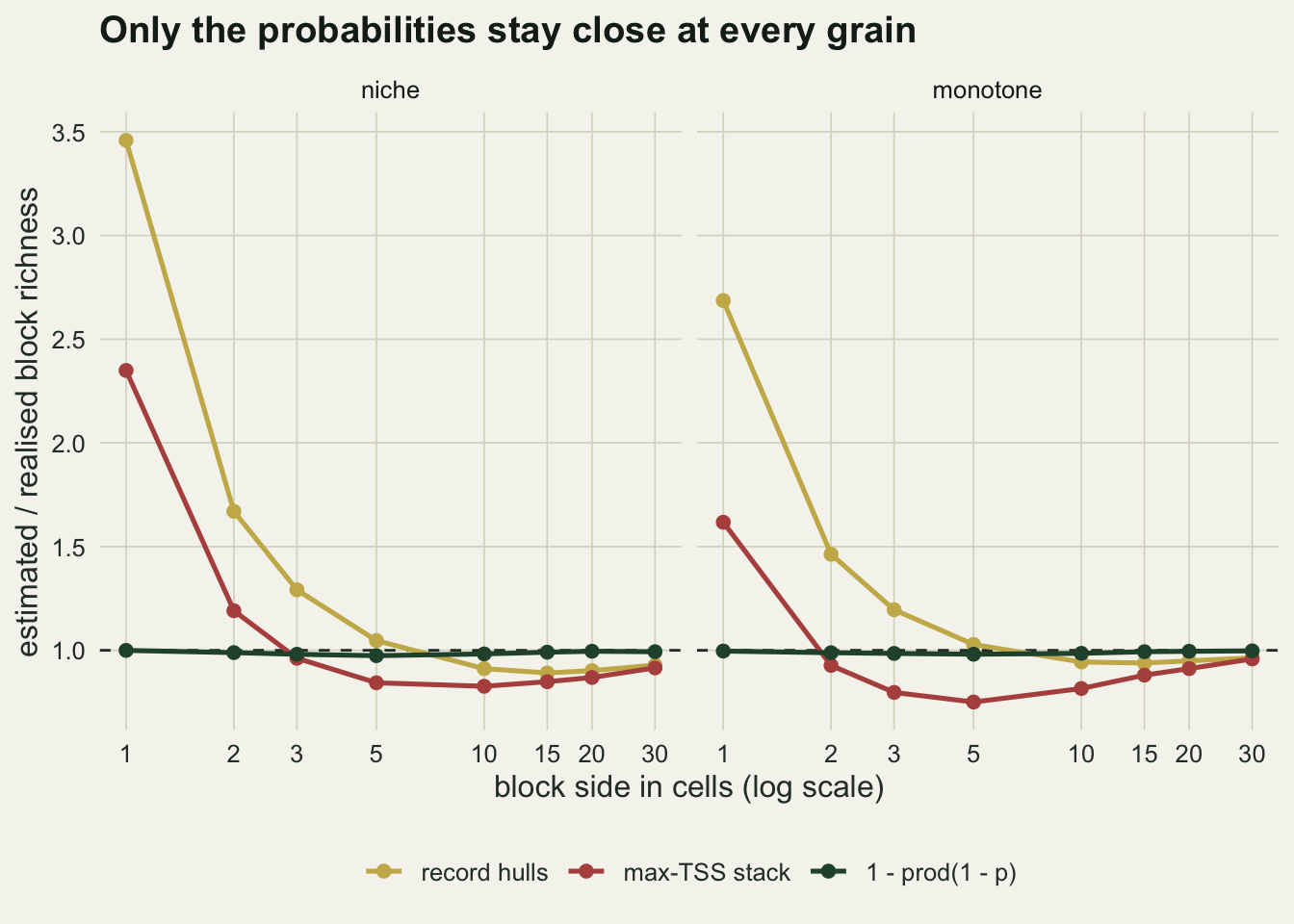
What to report
Map the sum of the fitted probabilities as the richness estimate, and say that it is an expected count, which needs calibrated models but not independent species. If a decision needs a binary map, threshold the richness surface or the conservation score that uses it, not each species before stacking; a per-species cut chosen for single-species accuracy was never meant to be added up.
If a binary stack has been published, state the threshold rule. At the grain of the model cells, and if the models are calibrated, expect the mean to be too high by the sum over species written above, which can be computed from the fitted probabilities and the cuts without any new data. Expect the contrast between rich and poor cells to be exaggerated as well. If the binary cells have been merged into coarser blocks the error can reverse: here the merged stack fell below realised block richness from blocks of 3 by 3 cells in the niche worlds and 2 by 2 in the monotone ones.
Report the grain at which richness is mapped, and aggregate to coarser blocks with 1 - prod(1 - p) per species, which assumes independence between cells, not by summing cell values and not by merging binary cells. Range-map hulls belong at coarse grain only, and even there they undercount when they are built from a small survey.
Give the Poisson-binomial interval with the independence assumption stated beside it. On held-out survey plots compare the squared gap between observed richness and the summed probabilities with the Poisson-binomial variance; a ratio well above one means the species share variation the models do not see, or that the models are miscalibrated, and either way the interval is too narrow.
The summed probabilities are only as good as the calibration of each model. A model whose probabilities are too high or too low passes its error straight into the sum; calibrating predicted probabilities in R shows how to check that per species before stacking.
Honest limits
Detection is perfect: every surveyed cell records every species present. With imperfect detection the fitted probabilities are probabilities of being recorded, and their sum estimates recorded richness, not true richness.
The fitted models have the right form. In the niche worlds the logistic regression with squared terms is the true model, and in the monotone worlds it nests it. A misspecified or miscalibrated model breaks the unbiasedness of the sum, and nothing above measures by how much. Calabrese and colleagues (2014) found that correctly stacked models of real data over-predicted richness at species-poor sites and under-predicted it at species-rich ones, a compressed contrast that the correctly specified models here do not show; they suggested regression dilution, covariates that describe a whole grid cell rather than the habitat a species uses, as a cause, and the covariates here are known without error.
Species are independent given the covariates in the main runs, and the shared site effect is independent between cells. Occurrences are independent between cells given the probabilities; clumped occurrences would make 1 - prod(1 - p) over-predict block richness, by an amount not measured here. A spatially smooth unmeasured driver would add spatial structure to the errors of the summed map, which was not simulated.
The hulls are built from the survey presences alone. Published range maps are drawn by experts from many sources, buffered, trimmed to habitat and edited; their grain behaviour may differ in detail from these hulls, although the arithmetic at single cells is the same for any polygon.
The species pools are drawn from one set of distributions for peak, width and optimum, on one grid of 3600 cells with one survey size. The size of the max-TSS excess depends on the prevalence mix, so the factors reported here are properties of these pools, not constants.
References
Calabrese JM, Certain G, Kraan C, Dormann CF 2014 Global Ecology and Biogeography 23(1):99-112 (10.1111/geb.12102)
Hurlbert AH, Jetz W 2007 Proceedings of the National Academy of Sciences 104(33):13384-13389 (10.1073/pnas.0704469104)
Allouche O, Tsoar A, Kadmon R 2006 Journal of Applied Ecology 43(6):1223-1232 (10.1111/j.1365-2664.2006.01214.x)