library(ggplot2)
library(patchwork)
library(nlme)

te_paper  <- "#f5f4ee"
te_ink    <- "#16241d"
te_body   <- "#2c3a31"
te_forest <- "#275139"
te_rust   <- "#b5534e"
te_gold   <- "#c9b458"
te_line   <- "#dad9ca"

theme_datasheet <- function() {
  theme_minimal(base_size = 12) +
    theme(plot.background  = element_rect(fill = te_paper, colour = NA),
          panel.background = element_rect(fill = te_paper, colour = NA),
          panel.grid.major = element_line(colour = te_line, linewidth = 0.3),
          panel.grid.minor = element_blank(),
          text             = element_text(colour = te_body),
          plot.title       = element_text(colour = te_ink, face = "bold"),
          plot.subtitle    = element_text(colour = te_body),
          axis.text        = element_text(colour = te_body),
          strip.text       = element_text(colour = te_ink))
}
class_cols <- c(resident = te_forest, nomad = te_line, dispersal = te_gold, migrant = te_rust)Classifying migrants from net squared displacement
R
movement ecology
migration
model selection
simulation
ecology tutorial
Choosing net squared displacement curves by AIC labels stationary home-range residents as migrants more often the slower they roam. Floors and AR(1) fits in R.
A herd of red deer winters low in a mountain valley, and twenty hinds carry GPS collars fitted in January. Each collar takes one fix a day for a year. Some of the hinds will climb to summer range in May and come back in the autumn, some will stay put, and the report needs a number: the proportion of the population that migrates. The standard way to get it is to turn each animal-year into a single series, the net squared displacement from the first fix, fit a small family of curves to it and let an information criterion pick the curve. A plateau is a resident, a single step is a disperser, a step up and a step back down is a migrant, a straight line is a nomad.
That model set is Bunnefeld and colleagues’ 2011 approach, and the migrateR package of Spitz, Hebblewhite and Stephenson packages it with a set of constraints on the fitted parameters. Singh, Allen and Ericsson wrote a paper of clarifications and caveats for the approach, including that short-distance migrants can be classified as residents or nomads, and Cagnacci and colleagues compared it with other ways of assessing migration on the same data. None of that is new here. What this post measures is the other side of the error: how often a hind that never left her range is called a migrant, and what sets the rate.
This site has three posts that touch the pieces. Correlated random walks and net displacement uses net squared displacement as a diffusion null, and because a single walk is noisy it averages the curve over a thousand replicate walks before reading it. A collar gives one walk per animal per year, and the classification is made on that one noisy series. Home ranges in R: MCP versus kernel density simulates a range as an Ornstein-Uhlenbeck process and shows that the autocorrelation time, roughly how long the animal takes to forget where it was, sets how much a track can say about the range. That time scale turns out to be the whole story below. Brownian motion or Ornstein-Uhlenbeck? counts how often an information criterion prefers the richer model on data from the simpler one, on phylogenies; the same kind of count is made here on tracks, where the richer models are the migrant and disperser curves.
The residents are simulated as a stationary Ornstein-Uhlenbeck range, so the true answer is always resident and every other label is an error. The post fits the four curves carefully, counts how the choice depends on the range’s autocorrelation time, and then tries three repairs: a stricter criterion, the displacement floor that migrateR offers, and autocorrelated errors in the curve fit.
Four curves for one animal-year
day      <- 0:364                   # one daily fix per day, first fix on day 0
n_fix    <- length(day)
s_km     <- 1                       # stationary SD of the range on each axis, km
tau_set  <- c(1, 3, 7, 15, 30, 60)  # position autocorrelation time, days
n_res    <- 200                     # resident animal-years per tau
tau_mig  <- 15                      # tau for the migrant runs
dist_set <- c(1, 2, 4, 8)             # migration distance, km
n_mig    <- 200                     # migrant animal-years per distance
leave_day <- 120; return_day <- 270; move_phi <- 5
floor_set <- c(3, 5)                # displacement floors, km
tau_ar   <- c(3, 15, 60)            # tau for the AR(1) refits
n_ar     <- 200                     # residents refitted per tau

r95_km   <- sqrt(qchisq(0.95, 2)) * s_km   # radius holding 95 per cent of positions

logistic <- function(theta, phi) 1 / (1 + exp((theta - day) / phi))

# 2-D OU around a fixed centre by its exact daily update, plus an optional
# seasonal shift of the centre along x; NSD is measured from the first fix
sim_nsd <- function(tau, s = s_km, dist = 0) {
  a <- exp(-1 / tau)
  ou_axis <- function() as.numeric(stats::filter(rnorm(n_fix, 0, s * sqrt(1 - a^2)), a,
                                    method = "recursive", init = rnorm(1, 0, s)))
  x <- ou_axis() + dist * (logistic(leave_day, move_phi) - logistic(return_day, move_phi))
  y <- ou_axis()
  (x - x[1])^2 + (y - y[1])^2
}
A resident hind is a two-dimensional Ornstein-Uhlenbeck process around a fixed centre: on each axis her position is pulled back towards the centre with time constant tau, and her stationary distribution has a standard deviation of 1 km on each axis, so 95 per cent of her positions lie within 2.45 km of the centre. Fleming and colleagues treat this time scale as the range crossing time, roughly how long the animal takes to cross its range. It runs from 1 to 60 days in the design, from an animal that crosses its range every day or two to one that spends weeks in one corner before drifting to another. A migrant is the same process whose centre moves 1 to 8 km along one axis in a logistic step around day 120 and back around day 270. The daily update is exact, so the tracks carry no discretisation error, and the first fix is drawn from the stationary distribution, so the collar starts wherever the animal happens to be. All of these constants, and the numbers of simulated animal-years, were fixed before the first run.
The four curves are the ones in Bunnefeld and colleagues’ paper, written for net squared displacement (NSD) against day. The nomad is a straight line through the origin. The resident rises to a plateau delta as one minus a negative exponential. The disperser is a logistic step of height delta at day theta with width phi. The migrant is a logistic step up at theta minus a step of the same height down at theta2, each with its own width, and, as in the migrateR parameterisation, the midpoint of the return lies at least twice the sum of the two widths after the midpoint of the departure. The mixed migrant curve, which returns to a different place, is left out.
Fitting the curves without failed fits
Fitting these curves with nls needs starting values, and a fit that stops with an error quietly becomes a missing model, which changes the choice. The fits here avoid that by the shape of the models. Every curve is delta times a shape that does not involve delta, so for any fixed shape the least squares delta has a closed form, truncated at zero. The fit is then a search over the shape parameters alone: a grid of shapes gives starting points, and Nelder-Mead runs from the three best grid shapes, twice each, polish the fit. Nothing in that search can stop with an error, so no animal-year is ever missing a model.
n_par <- c(nomad = 1, resident = 2, dispersal = 3, migrant = 5)  # excluding sigma

# curve shapes without delta; p on the optimiser scale (log rates and log phi)
shape_of <- function(model, p) switch(model,
  resident  = 1 - exp(-exp(p[1]) * day),
  dispersal = logistic(p[1], exp(p[2])),
  migrant   = logistic(p[1], exp(p[3])) - logistic(p[2], exp(p[4])))
valid_par <- function(model, p) model != "migrant" ||
  p[2] >= p[1] + 2 * exp(p[3]) + 2 * exp(p[4])

rho_set <- c(0, seq(0.05, 0.995, length.out = 60))

# least squares for delta >= 0 given the shape; with ar = TRUE the errors are
# AR(1), fitted by conditional least squares with rho profiled over rho_set
profile_delta <- function(X, y, ar = FALSE) {
  X <- as.matrix(X)
  if (!ar) {
    xy <- crossprod(X, y)[, 1]; xx <- colSums(X^2); dl <- pmax(xy / xx, 0)
    return(list(rss = sum(y^2) - 2 * dl * xy + dl^2 * xx, delta = dl, rho = rep(0, ncol(X))))
  }
  X1 <- X[-1, , drop = FALSE]; X0 <- X[-n_fix, , drop = FALSE]
  y1 <- y[-1]; y0 <- y[-n_fix]
  c11 <- crossprod(X1, y1)[, 1]; c10 <- crossprod(X1, y0)[, 1]
  c01 <- crossprod(X0, y1)[, 1]; c00 <- crossprod(X0, y0)[, 1]
  s11 <- colSums(X1^2); s10 <- colSums(X1 * X0); s00 <- colSums(X0^2)
  q11 <- sum(y1^2); q10 <- sum(y1 * y0); q00 <- sum(y0^2)
  rss <- rep(Inf, ncol(X)); dl <- rho <- rep(0, ncol(X))
  for (r in rho_set) {
    xy <- c11 - r * (c10 + c01) + r^2 * c00
    xx <- s11 - 2 * r * s10 + r^2 * s00
    dd <- pmax(xy / xx, 0)
    rr <- q11 - 2 * r * q10 + r^2 * q00 - 2 * dd * xy + dd^2 * xx
    better <- rr < rss
    rss[better] <- rr[better]; dl[better] <- dd[better]; rho[better] <- r
  }
  list(rss = rss, delta = dl, rho = rho)
}

# starting grids on the optimiser scale, one shape per column
start_grid <- list(
  resident  = cbind(log(exp(seq(log(0.003), log(3), length.out = 40)))),
  dispersal = as.matrix(expand.grid(seq(5, 360, 5), log(c(1, 3, 7, 15, 30)))),
  migrant   = local({
    g <- as.matrix(expand.grid(seq(10, 350, 10), seq(10, 350, 10), log(c(2, 6, 15)), log(c(2, 6, 15))))
    g[apply(g, 1, function(p) valid_par("migrant", p)), ]
  }))
start_shape <- lapply(names(start_grid), function(m)
  apply(start_grid[[m]], 1, function(p) shape_of(m, p)))
names(start_shape) <- names(start_grid)

# one shape at a time, with the sums over the track computed once per track
rss_shape <- function(x, trk, ar) {
  if (!ar) {
    xy <- sum(x * trk$y); xx <- sum(x * x); dl <- max(xy / xx, 0)
    return(c(trk$yy - 2 * dl * xy + dl^2 * xx, dl, 0))
  }
  x1 <- x[-1]; x0 <- x[-n_fix]; r <- rho_set
  xy <- sum(x1 * trk$y1) - r * (sum(x1 * trk$y0) + sum(x0 * trk$y1)) + r^2 * sum(x0 * trk$y0)
  xx <- sum(x1 * x1) - 2 * r * sum(x1 * x0) + r^2 * sum(x0 * x0)
  dl <- pmax(xy / xx, 0); rr <- trk$q - 2 * dl * xy + dl^2 * xx; i <- which.min(rr)
  c(rr[i], dl[i], r[i])
}

# grid start, then Nelder-Mead from the three best grid shapes, run twice each
fit_curve <- function(model, y, ar = FALSE, n_start = 3) {
  trk <- list(y = y, yy = sum(y^2), y1 = y[-1], y0 = y[-n_fix])
  trk$q <- sum(trk$y1^2) - 2 * rho_set * sum(trk$y1 * trk$y0) + rho_set^2 * sum(trk$y0^2)
  if (model == "nomad") {
    v <- rss_shape(day, trk, ar)
    return(list(rss = v[1], delta = v[2], rho = v[3], par = numeric(0), top = v[2] * max(day)))
  }
  pr <- profile_delta(start_shape[[model]], y, ar)
  objective <- function(p) {
    if (!valid_par(model, p) || any(abs(p) > 1000)) return(.Machine$double.xmax)
    rss_shape(shape_of(model, p), trk, ar)[1]
  }
  best <- Inf; best_par <- NULL
  for (i in order(pr$rss)[seq_len(if (model == "resident") 1 else n_start)]) {
    if (model == "resident") {
      par <- optimize(objective, log(c(1e-4, 20)))$minimum
    } else {
      par <- start_grid[[model]][i, ]
      for (run in 1:2) par <- optim(par, objective, control = list(maxit = 400))$par
    }
    v <- rss_shape(shape_of(model, par), trk, ar)
    if (v[1] < best[1]) { best <- v; best_par <- par }
  }
  list(rss = best[1], delta = best[2], rho = best[3], par = best_par,
       top = best[2] * max(shape_of(model, best_par)))
}

fit_year <- function(y, ar = FALSE) {
  fits <- lapply(names(n_par), fit_curve, y = y, ar = ar)
  names(fits) <- names(n_par)
  c(sapply(fits, `[[`, "rss"), sapply(fits, `[[`, "delta"), sapply(fits, `[[`, "top"), ar = ar)
}

# the choice; floor_km removes dispersal and migrant fits with delta below
# floor_km^2 (migrateR's mdelta); nomad_rule also removes the nomad fit when its
# largest fitted NSD is within floor_km^2 of the resident's (migrateR's mnr);
# parsimony takes the fewest parameters within 2 AIC units (migrateR's a.rule)
choose_model <- function(fr, pen = 2, floor_km = 0, nomad_rule = FALSE, parsimony = FALSE) {
  ar <- fr[["ar"]]; m_obs <- n_fix - ar
  ic <- m_obs * log(fr[1:4] / m_obs) + pen * (n_par + 1 + ar)
  keep <- c(TRUE, TRUE, fr[7:8] >= floor_km^2)
  if (nomad_rule) keep[1] <- abs(fr[[10]] - fr[[9]]) >= floor_km^2
  ic[!keep] <- Inf
  pick <- which.min(ic)
  if (parsimony) pick <- which(ic - min(ic) <= 2)[1]   # n_par is in increasing order
  names(n_par)[pick]
}
The same device gives a fit with AR(1) errors. For a fixed shape and a fixed autocorrelation rho the conditional least squares problem is again linear in delta, so rho is profiled over a grid of values from zero to 0.995 inside the same search, and the criterion counts rho as one more parameter.
The choice itself is a function of the fitted residual sums of squares and the two migrateR rules. Its displacement floor drops a disperser or migrant fit whose delta is below a minimum; since delta is in squared km, a floor of 3 km means delta below 9. Nomads have no delta, so the floor never touches them; migrateR has a separate rule for them, which drops the nomad fit when its largest fitted NSD differs from the largest fitted NSD of the resident curve by less than a set amount, here the same squared floor. By default migrateR also takes the model with the fewest parameters among those within 2 AIC units of the best, which is included as a third variant of the criterion.
set.seed(4417)
chk_y <- replicate(40, sim_nsd(30))
chk_nls <- t(apply(chk_y, 2, function(y) {
  out <- c()
  for (m in c("dispersal", "migrant")) {
    pr <- profile_delta(start_shape[[m]], y); i <- which.min(pr$rss); p0 <- start_grid[[m]][i, ]
    dat <- data.frame(dday = day, nsd = y)
    fm <- if (m == "dispersal") {
      try(nls(nsd ~ delta / (1 + exp((theta - dday) / phi)), dat,
              start = list(delta = pr$delta[i], theta = p0[[1]], phi = exp(p0[[2]]))), silent = TRUE)
    } else {
      try(nls(nsd ~ delta / (1 + exp((theta - dday) / phi)) - delta / (1 + exp((theta2 - dday) / phi2)), dat,
              start = list(delta = pr$delta[i], theta = p0[[1]], theta2 = p0[[2]],
                           phi = exp(p0[[3]]), phi2 = exp(p0[[4]]))), silent = TRUE)
    }
    nls_rss <- if (inherits(fm, "try-error")) NA else deviance(fm)
    out <- c(out, nls_rss, fit_curve(m, y)$rss)
  }
  out
}))
nls_fail  <- colSums(is.na(chk_nls[, c(1, 3)]))
nm_gain   <- n_fix * log(chk_nls[, c(1, 3)] / chk_nls[, c(2, 4)])   # AIC units, NA if nls failed
nls_beats <- colSums(nm_gain < -0.01, na.rm = TRUE)   # nls found a lower RSS
nm_worst  <- -apply(nm_gain, 2, min, na.rm = TRUE)    # largest shortfall, AIC units
n_chk     <- ncol(chk_y)

# the AR(1) profile against nlme::gnls with corAR1, dispersal curve, ten tracks
gn_out <- t(sapply(1:10, function(j) {
  pf <- fit_curve("dispersal", chk_y[, j], ar = TRUE)
  fm <- try(gnls(nsd ~ delta / (1 + exp((theta - dday) / phi)),
                 data.frame(dday = day, nsd = chk_y[, j]),
                 start = c(delta = pf$delta, theta = pf$par[[1]], phi = exp(pf$par[[2]])),
                 correlation = corAR1(form = ~ dday)), silent = TRUE)
  if (inherits(fm, "try-error")) return(c(NA, pf$rho, NA, pf$delta))
  c(coef(fm$modelStruct$corStruct, unconstrained = FALSE)[[1]], pf$rho, coef(fm)[["delta"]], pf$delta)
}))
gn_fail  <- sum(is.na(gn_out[, 1]))
gn_rho_gap   <- max(abs(gn_out[, 1] - gn_out[, 2]), na.rm = TRUE)
gn_delta_gap <- max(abs(gn_out[, 3] / gn_out[, 4] - 1), na.rm = TRUE)

# scale: the same random numbers with a range half and twice as wide
set.seed(918); y_half <- replicate(20, sim_nsd(15, s = 0.5))
set.seed(918); y_twice <- replicate(20, sim_nsd(15, s = 2))
fr_half  <- apply(y_half, 2, fit_year); fr_twice <- apply(y_twice, 2, fit_year)
same_class <- mean(apply(fr_half, 2, choose_model) == apply(fr_twice, 2, choose_model))
delta_ratio <- range(fr_twice[8, ] / fr_half[8, ])
The checks come before the results. The first compares the search with nls, started from the best grid shape, on 40 resident tracks with tau of 30 days. For the disperser nls failed on 2 tracks and found a lower residual sum of squares than the search on 0 of the others. For the migrant nls failed on 21 of the 40 tracks. Where it converged it found a lower residual sum of squares on 6 tracks, by at most 2.6 AIC units. A migrant fit that falls short makes a migrant choice less likely, so if anything the search slightly understates the false migrant rates that follow.
The second fits the AR(1) disperser with nlme::gnls and a corAR1 structure on the first ten of the same tracks, starting from the profile fit. gnls stopped with an error on 5 of them. On the rest its rho differed from the profile by at most 0.011 and its delta by at most 9 per cent, a gap plausibly due to the conditional least squares used here against the full likelihood in gnls.
The last check is on scale rather than on the optimiser. Multiplying every position by a constant c multiplies every NSD by c squared and every residual sum of squares by c to the fourth power, which leaves every AIC difference unchanged. The same random numbers with a range half as wide and twice as wide gave the same class for 100 per cent of 20 tracks, and delta ratios of 16 to 16. Without a floor the choice depends on tau and on the migration distance over the range size, never on the range size alone. With a floor it depends on the floor over the range size, which matters for the floor section below.
Residents turn into migrants as tau grows
set.seed(20260917)
res_y  <- lapply(tau_set, function(tau) replicate(n_res, sim_nsd(tau)))
res_fr <- lapply(res_y, function(ym) apply(ym, 2, fit_year))

share_tab <- function(fr_list, keys, rule, ...) {
  do.call(rbind, lapply(seq_along(fr_list), function(i) {
    cl <- apply(fr_list[[i]], 2, choose_model, ...)
    data.frame(key = keys[i], class = names(n_par), rule = rule,
               share = as.numeric(table(factor(cl, levels = names(n_par)))) / ncol(fr_list[[i]]))
  }))
}
get_share <- function(tab, rule_name, cls) tab$share[tab$rule == rule_name & tab$class == cls]
mc_se <- function(p, nn) sqrt(p * (1 - p) / nn)

res_share <- rbind(share_tab(res_fr, tau_set, "AIC"),
                   share_tab(res_fr, tau_set, "AIC, parsimony rule", parsimony = TRUE),
                   share_tab(res_fr, tau_set, "BIC", pen = log(n_fix)))
aic_ok  <- get_share(res_share, "AIC", "resident")
par_ok  <- get_share(res_share, "AIC, parsimony rule", "resident")
bic_ok  <- get_share(res_share, "BIC", "resident")
aic_mig <- get_share(res_share, "AIC", "migrant")
aic_dis <- get_share(res_share, "AIC", "dispersal")
nomad_max <- max(res_share$share[res_share$class == "nomad"])
se_max  <- max(mc_se(c(aic_ok, par_ok, bic_ok), n_res))

# the same tracks classified from the starting grid alone, without the polish
grid_year <- function(y) {
  fits <- lapply(names(n_par), function(m) {
    pr <- if (m == "nomad") profile_delta(day, y) else profile_delta(start_shape[[m]], y)
    i <- which.min(pr$rss); c(pr$rss[i], pr$delta[i])
  })
  c(sapply(fits, `[`, 1), sapply(fits, `[`, 2), rep(0, 4), ar = 0)
}
i15 <- match(15, tau_set)
grid_ok <- mean(apply(apply(res_y[[i15]], 2, grid_year), 2, choose_model) == "resident")
With AIC, the share of residents classified as residents was 0.795 at tau of 1 day, 0.470 at 3 days, 0.120 at 15 days and 0.020 at 60 days, from 200 animal-years per value with Monte Carlo standard errors of 0.035 or less. At tau of 60 days the migrant curve won for 0.690 of the residents and the disperser for 0.285. Nomads were almost never chosen: the largest nomad share in any cell, under any of the three criteria, was 0.005.
The error at the short end is not zero either. At a tau of one day, positions a day apart keep a correlation of only 0.37, and still 0.205 of those residents were given a sigmoid curve. A plausible reason is that the timing parameters of the sigmoid curves act like change points, which can buy more fit than the 2 AIC units each is charged, and that NSD measured from one fix is a skewed series whose spread changes with its level, for which a least squares criterion is only an approximation.
The parsimony rule of migrateR raised the resident share to 0.190 at 15 days, and BIC, whose penalty per parameter is 5.9 for a year of daily fixes, to 0.345. BIC kept 0.985 of the residents at 1 day and 0.860 at 3 days, but by 60 days it keeps only 0.080 of the residents. No penalty that is fixed per parameter can follow tau, because the extra fit a wandering resident offers the migrant curve grows with tau while the penalty does not.
The optimiser matters in the direction nobody would pick. Classifying the same 200 residents at tau of 15 days from the starting grid alone, without the Nelder-Mead polish, kept 0.345 of them as residents against 0.120 with it. A coarse fit to the flexible curves flatters the method; the better the curves are fitted, the more false migrants appear.
plot_share <- res_share
plot_share$class <- factor(plot_share$class, levels = c("migrant", "dispersal", "nomad", "resident"))
plot_share$tau <- factor(plot_share$key, levels = tau_set)
ggplot(plot_share, aes(tau, share, fill = class)) +
  geom_col(width = 0.75, colour = te_paper, linewidth = 0.2) +
  facet_wrap(~ rule) +
  scale_fill_manual(values = class_cols, name = "label") +
  scale_y_continuous(breaks = seq(0, 1, 0.25)) +
  labs(x = "range autocorrelation time tau (days)", y = "share of residents",
       title = "Stationary residents labelled by curve choice",
       subtitle = sprintf("%d animal-years per bar, daily fixes for a year", n_res)) +
  theme_datasheet() +
  theme(legend.position = "bottom")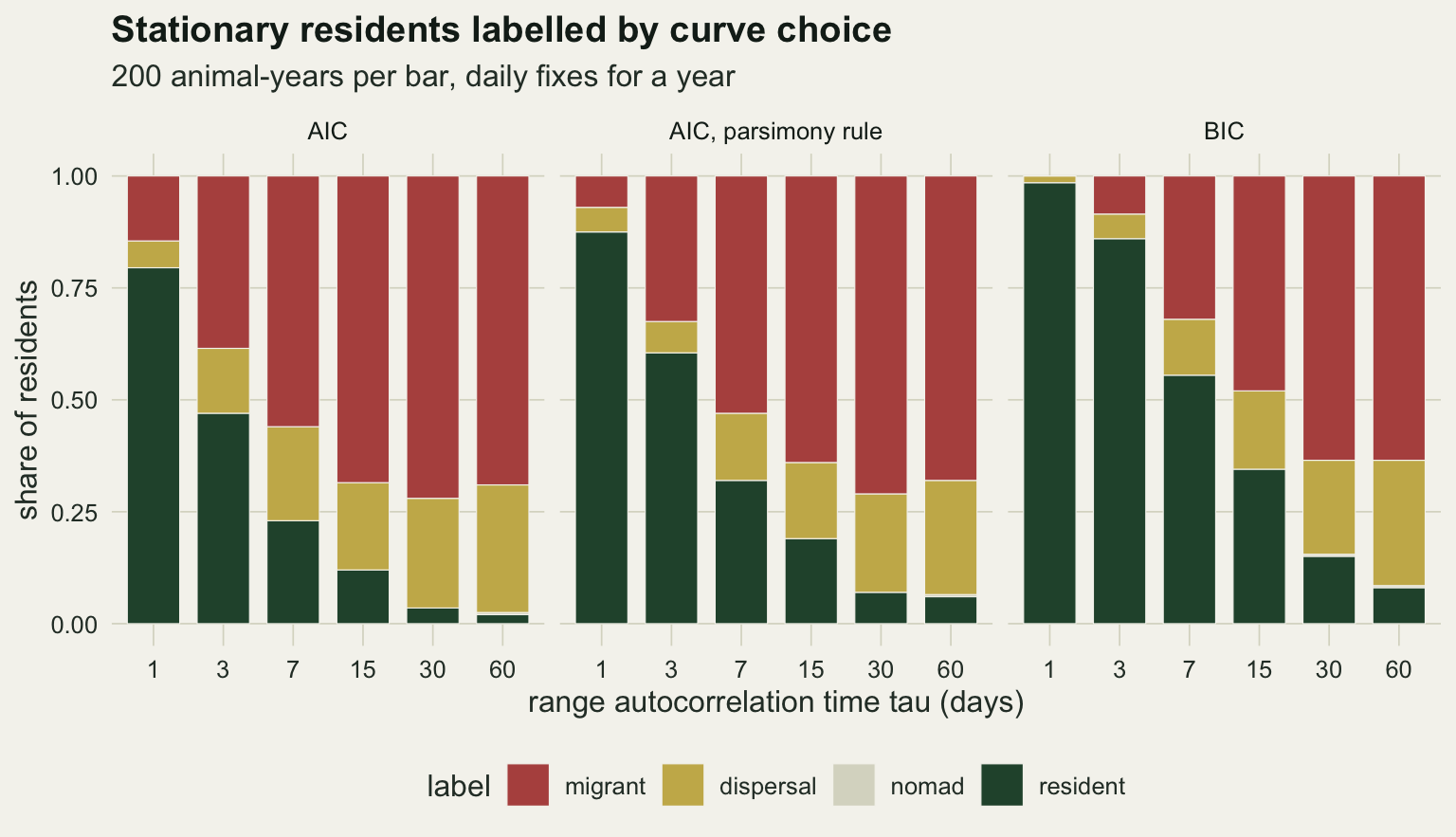
example_panel <- function(y, lab) {
  fr <- fit_year(y); pick <- choose_model(fr)
  fc <- fit_curve(pick, y)
  shape <- if (pick == "nomad") day else shape_of(pick, fc$par)
  list(pts = data.frame(day = day, nsd = y, panel = lab),
       fit = data.frame(day = day, nsd = fc$delta * shape, panel = lab, pick = pick))
}
ex <- list(example_panel(res_y[[1]][, 1], sprintf("resident, tau %d d", tau_set[1])),
           example_panel(res_y[[5]][, 1], sprintf("resident, tau %d d", tau_set[5])))
set.seed(33)
ex[[3]] <- example_panel(sim_nsd(tau_mig, dist = 4), sprintf("migrant 4 km, tau %d d", tau_mig))
ex_pts <- do.call(rbind, lapply(ex, `[[`, "pts"))
ex_fit <- do.call(rbind, lapply(ex, `[[`, "fit"))
ex_lab <- unique(ex_fit[, c("panel", "pick")])
ex_pts$panel <- factor(ex_pts$panel, levels = unique(ex_pts$panel))
ex_fit$panel <- factor(ex_fit$panel, levels = levels(ex_pts$panel))
ex_lab$panel <- factor(ex_lab$panel, levels = levels(ex_pts$panel))
ggplot(ex_pts, aes(day, nsd)) +
  geom_point(size = 0.6, colour = te_body, alpha = 0.45) +
  geom_line(data = ex_fit, aes(colour = pick), linewidth = 1.1) +
  geom_label(data = ex_lab, aes(x = 5, y = Inf, label = paste("AIC choice:", pick)),
             hjust = 0, vjust = 1.3, size = 3.4, fill = te_paper, colour = te_ink) +
  facet_wrap(~ panel, scales = "free_y") +
  scale_colour_manual(values = class_cols, guide = "none") +
  labs(x = "day of the collar year", y = "NSD from the first fix (km squared)",
       title = "One animal-year, one curve") +
  theme_datasheet()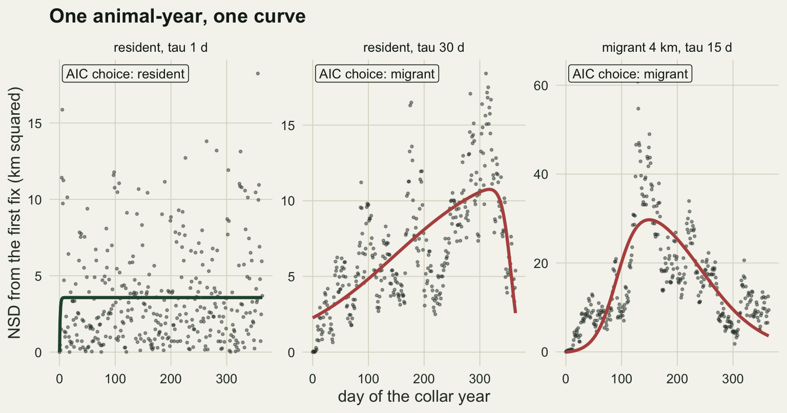
The example panels show why the flexible curves win. A resident with a long autocorrelation time spends weeks in one part of her range before drifting to another, so her distance from the first fix wanders in slow swings instead of scattering around a plateau. In the middle panel it climbs through most of the year and drops near the end, and a wide step up with a late step down describes that better than any plateau.
A displacement floor, and what it costs
A floor asks for a minimum size of the step before a sigmoid curve may win. The scale check above says what a floor in km really is: a floor in units of the range. For this range, 95 per cent of positions lie within 2.45 km of the centre, so the floors of 3 and 5 km are 1.2 and 2.0 times that radius; the same floors on a range twice as wide would be half as strict. The migrants were run at tau of 15 days, 200 animal-years per distance.
floor_res <- rbind(
  share_tab(res_fr, tau_set, "no floor"),
  share_tab(res_fr, tau_set, "3 km floor", floor_km = floor_set[1]),
  share_tab(res_fr, tau_set, "5 km floor", floor_km = floor_set[2]),
  share_tab(res_fr, tau_set, "5 km floor and nomad rule", floor_km = floor_set[2], nomad_rule = TRUE))
f3_ok  <- get_share(floor_res, "3 km floor", "resident")
f5_ok  <- get_share(floor_res, "5 km floor", "resident")
f5_nom <- get_share(floor_res, "5 km floor", "nomad")
f5n_ok <- get_share(floor_res, "5 km floor and nomad rule", "resident")

set.seed(170926)
mig_y  <- lapply(dist_set, function(dd) replicate(n_mig, sim_nsd(tau_mig, dist = dd)))
mig_fr <- lapply(mig_y, function(ym) apply(ym, 2, fit_year))
floor_mig <- rbind(
  share_tab(mig_fr, dist_set, "no floor"),
  share_tab(mig_fr, dist_set, "3 km floor", floor_km = floor_set[1]),
  share_tab(mig_fr, dist_set, "5 km floor", floor_km = floor_set[2]),
  share_tab(mig_fr, dist_set, "5 km floor and nomad rule", floor_km = floor_set[2], nomad_rule = TRUE))
m0_hit  <- get_share(floor_mig, "no floor", "migrant")
m3_hit  <- get_share(floor_mig, "3 km floor", "migrant")
m5_hit  <- get_share(floor_mig, "5 km floor", "migrant")
m5_res  <- get_share(floor_mig, "5 km floor", "resident")
m5n_hit <- get_share(floor_mig, "5 km floor and nomad rule", "migrant")
Among residents at tau of 15 days, where AIC alone kept 0.120, the 3 km floor kept 0.800 and the 5 km floor 0.945. At 60 days the numbers were 0.020, 0.580 and 0.770. The floor removes sigmoid fits, and some of those animal-years then fall to the nomad line instead of the resident curve: with the 5 km floor the nomad share at 60 days was 0.135, against almost none without it. Adding the nomad rule at the same distance put the resident share back to 0.905. A floor that is not also applied to the nomad model moves part of the error to a different wrong label.
The cost falls on short migrants. Without a floor AIC labelled 0.820 of the 2 km migrants as migrants, 0.990 of the 4 km migrants and 1.000 of the 8 km migrants. The 3 km floor left 0.445, 0.950 and 1.000; the 5 km floor left 0.050, 0.485 and 1.000, and the lost 4 km migrants went to resident (0.515). A fitted delta is a squared distance measured from a first fix that is itself somewhere in the winter range, so it scatters around the square of the true distance, and a floor near the true distance removes a large part of the migrants at that distance.
The 1 km migrants are a warning about the whole table rather than about the floor. Their step is well inside the winter range, and without a floor 0.700 of them were called migrants, against 0.685 of the stationary residents at the same tau. At that distance the migrant label says almost nothing about whether the animal moved.
rule_cols <- c("no floor" = te_rust, "3 km floor" = te_gold,
               "5 km floor" = te_forest, "5 km floor and nomad rule" = te_ink)
res_line <- floor_res[floor_res$class == "resident", ]
mig_line <- floor_mig[floor_mig$class == "migrant", ]
p_res <- ggplot(res_line, aes(key, share, colour = rule)) +
  geom_line(linewidth = 0.8) + geom_point(size = 1.8) +
  scale_x_log10(breaks = tau_set) +
  scale_colour_manual(values = rule_cols, breaks = names(rule_cols), name = NULL) +
  coord_cartesian(ylim = c(0, 1)) +
  labs(x = "tau (days, log scale)", y = "residents labelled resident", title = "Residents kept") +
  theme_datasheet()
p_mig <- ggplot(mig_line, aes(key, share, colour = rule)) +
  geom_line(linewidth = 0.8) + geom_point(size = 1.8) +
  scale_x_log10(breaks = dist_set) +
  scale_colour_manual(values = rule_cols, breaks = names(rule_cols), name = NULL) +
  coord_cartesian(ylim = c(0, 1)) +
  labs(x = "migration distance (km, log scale)", y = "migrants labelled migrant",
       title = "Migrants found") +
  theme_datasheet()
(p_res + p_mig) + plot_layout(guides = "collect") +
  plot_annotation(theme = theme_datasheet()) & theme(legend.position = "bottom")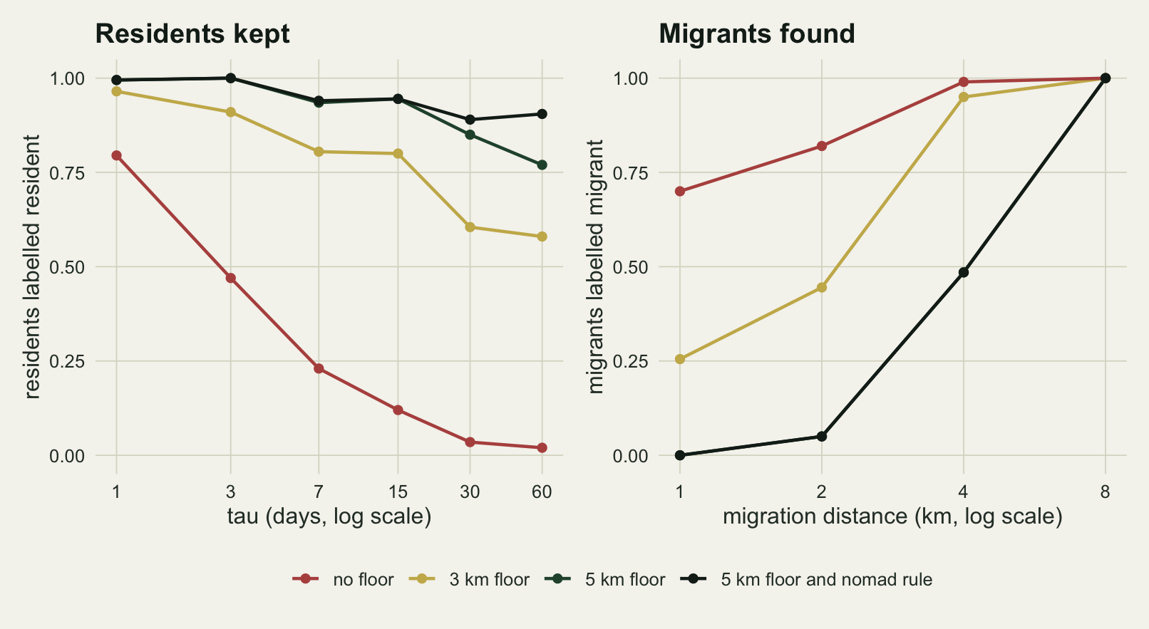
Autocorrelated errors do not restore the choice
The statistical complaint about the curve fits is that daily NSD values are treated as independent. The obvious repair keeps the curves and gives the errors an AR(1) structure, as gnls with corAR1 would. The residents at three values of tau were refitted that way, 200 animal-years each, so the comparison with the independent-error fits is paired.
ar_idx <- match(tau_ar, tau_set)
ar_fr  <- lapply(ar_idx, function(i) apply(res_y[[i]][, seq_len(n_ar)], 2, fit_year, ar = TRUE))
iid_fr <- lapply(ar_idx, function(i) res_fr[[i]][, seq_len(n_ar)])
ar_share <- rbind(share_tab(iid_fr, tau_ar, "independent errors, AIC"),
                  share_tab(iid_fr, tau_ar, "independent errors, BIC", pen = log(n_fix)),
                  share_tab(ar_fr, tau_ar, "AR(1) errors, AIC"),
                  share_tab(ar_fr, tau_ar, "AR(1) errors, BIC", pen = log(n_fix - 1)))
iid_ok   <- get_share(ar_share, "independent errors, AIC", "resident")
ar_ok    <- get_share(ar_share, "AR(1) errors, AIC", "resident")
arb_ok   <- get_share(ar_share, "AR(1) errors, BIC", "resident")
iidb_ok  <- get_share(ar_share, "independent errors, BIC", "resident")
ar_mig   <- get_share(ar_share, "AR(1) errors, AIC", "migrant")
ar_dis   <- get_share(ar_share, "AR(1) errors, AIC", "dispersal")
arb_nom  <- get_share(ar_share, "AR(1) errors, BIC", "nomad")
ar_se    <- max(mc_se(c(iid_ok, iidb_ok, ar_ok, arb_ok), n_ar))
At tau of 3 days the AR(1) fit kept 0.710 of the residents against 0.470 for the same tracks with independent errors, and with BIC 0.985 (independent errors with BIC: 0.860). At 15 days it kept 0.120 against 0.120; the migrant share fell to 0.435 but the disperser share rose to 0.420. At 60 days the resident share was 0.035 against 0.020. BIC with AR(1) errors kept 0.305 and 0.065 at the two longer time scales, against 0.345 and 0.080 with independent errors and BIC, so the AR(1) structure adds nothing there, and it sent 0.295 and 0.340 of the residents to the nomad line. Monte Carlo standard errors are 0.035 or less.
The AR(1) structure helps at the short time scale (with BIC, from 0.860 to 0.985) and not at the long ones, where its resident shares are slightly lower than with BIC alone. Most of the gain of AR(1) errors with BIC over independent errors with AIC comes from the penalty, not from the error structure. When rho is close to one, an AR(1) error series is itself almost a random walk, and a random walk and a slow excursion from the first fix are hard to separate from a trend: the label moves from migrant to disperser or to nomad rather than to resident. NSD from an Ornstein-Uhlenbeck range is also not an AR(1) series with constant variance; it is a squared distance whose spread grows with its level. A model that describes the positions themselves, a stationary range against a shifting one in continuous time, is the natural next step and is not tried here.
ar_plot <- ar_share
ar_plot$class <- factor(ar_plot$class, levels = c("migrant", "dispersal", "nomad", "resident"))
ar_plot$tau <- factor(sprintf("tau %d d", ar_plot$key), levels = sprintf("tau %d d", tau_ar))
ar_plot$rule <- factor(ar_plot$rule, levels = unique(ar_share$rule))
ggplot(ar_plot, aes(rule, share, fill = class)) +
  geom_col(width = 0.7, colour = te_paper, linewidth = 0.2) +
  facet_wrap(~ tau) +
  scale_fill_manual(values = class_cols, name = "label") +
  scale_x_discrete(labels = c("iid\nAIC", "iid\nBIC", "AR(1)\nAIC", "AR(1)\nBIC")) +
  labs(x = NULL, y = "share of residents",
       title = "AR(1) errors move the error, mostly",
       subtitle = sprintf("%d paired animal-years per tau", n_ar)) +
  theme_datasheet() +
  theme(legend.position = "bottom")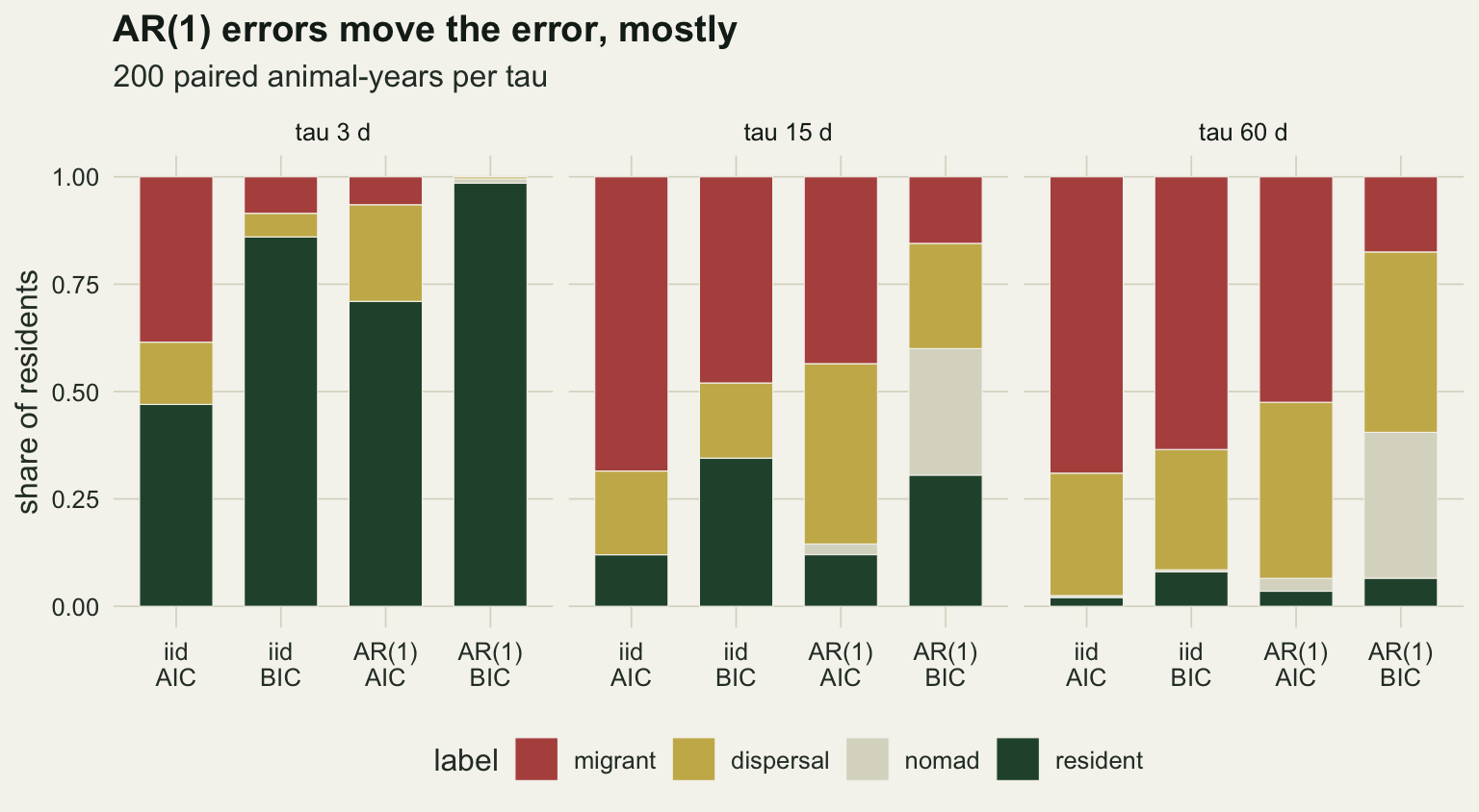
What to report
Report the curve set, the criterion and every constraint as numbers: the floor on delta in km and the range size it was compared against, whether the nomad model was held to a matching rule, and whether the parsimony rule was on. A floor stated in km means nothing without the range size, because without a floor the choice depends on the range size only through tau and the migration distance over the range size.
Estimate the autocorrelation time of the resident ranges from the positions before the classification, and say it. A share of migrants from a population whose residents cross their range in a day is not comparable with the same share from a population whose residents take a month, even with identical collars and identical code.
Simulate the population’s own residents. A stationary Ornstein-Uhlenbeck range with the estimated range size and tau, run through the same fitting and choice code, gives the false migrant rate for that study directly; the code above is enough for that. If the rate is not small, report the migrant share next to it, or treat the classification as a screen for animals whose tracks are then read by eye.
Keep a short-distance migrant category open. Where the migration distance is not well beyond the range radius, none of the rules measured here separates them from residents at tau of 15 days or more without losing most of them, and a floor large enough to protect the residents removes those migrants by construction.
Honest limits
Every resident here has a single stationary range with an isotropic, Gaussian Ornstein-Uhlenbeck process, and every migrant makes one symmetric trip with fixed dates. Real winter ranges drift, are shaped by terrain and snow, and have more than one centre; each of those adds structure that the sigmoid curves can take for movement, so there is no reason to expect real residents with the same tau to be misclassified less often than these.
The fixes are daily and perfect: no location error, no gaps, no four-hourly schedule. More fixes per day at the same tau add points without adding independent information, so a fixed penalty per parameter would be expected to do worse with them, but that was not run.
The first fix is the reference point throughout. Singh and colleagues discuss how the start date changes NSD classification, above all when the start falls inside a migration, and a start at the range centre instead of at a random position could change the resident rates. That is a separate lesson and was left out on purpose.
The criterion is least squares on NSD, as in the curve fits it copies. The mixed migrant curve is missing, the migrant’s timing constraint is the migrateR one without its further limits on timing, and the Nelder-Mead search sometimes stopped short of nls on the migrant curve, which the check above sized. The AR(1) repair was profiled over a grid of rho and fitted by conditional least squares, which agreed with gnls where gnls converged but is not identical to it.
Only one tau (15 days) was run for the migrants, the AR(1) refits covered three of the six values of tau, and the migrants were not refitted with AR(1) errors at all, to keep the page under a few minutes to build. What a floor or an AR(1) fit does to migrants with a long autocorrelation time is therefore not measured here. No true dispersers were simulated, so the disperser label is only ever an error here.
References
Bunnefeld N, Borger L, van Moorter B, Rolandsen CM, Dettki H, Solberg EJ, Ericsson G 2011 Journal of Animal Ecology 80(2):466-476 (10.1111/j.1365-2656.2010.01776.x)
Spitz DB, Hebblewhite M, Stephenson TR 2017 Ecography 40(6):788-799 (10.1111/ecog.02587)
Singh NJ, Allen AM, Ericsson G 2016 PLoS ONE 11(3):e0149594 (10.1371/journal.pone.0149594)
Cagnacci F, Focardi S, Ghisla A, van Moorter B, Merrill EH, Gurarie E, Heurich M, Mysterud A, Linnell J, Panzacchi M, May R, Nygard T, Rolandsen C, Hebblewhite M 2016 Journal of Animal Ecology 85(1):54-68 (10.1111/1365-2656.12449)
Fleming CH, Calabrese JM, Mueller T, Olson KA, Leimgruber P, Fagan WF 2014 American Naturalist 183(5):E154-E167 (10.1086/675504)