---
title: "SCR sampling design and precision"
description: "How trap spacing relative to sigma controls spatial recaptures and the precision of density in spatial capture-recapture, worked from scratch in base R."
date: "2026-05-20 13:00"
date-modified: "2026-11-06"
categories: [R, capture-recapture, spatial, study design, ecology tutorial]
image: thumbnail.png
image-alt: "Two lines of coefficient of variation against trap spacing in units of sigma. The dark green density line falls steeply from 0.5 at the tightest spacing to a low point labelled optimum near 2 sigma, then rises gently; the red sigma line sits lower, easing at first and then nearly flat."
---
*Corrected 7 October 2026: the introduction still said that wide spacing leaves sigma resting on a handful of spatial recaptures, and the section on the two forces said spatial recaptures are needed to fix the detection scale, although the sweep shows the sigma estimate about as precise at the widest spacing as at the optimum; both now say only that recaptures become rare there, the opening of the section on spatial recaptures now says the frequentist post leaned on them rather than that they alone pin down sigma, and the post now reports that at that spacing the density estimate is more strongly tied to the sigma estimate. The figure caption said density precision is worst at both extremes; it now says precision is worst at the tightest spacing and slips again at wider spacings.*
*Corrected 30 September 2026: the post called the lowest point of the precision curve a clear optimum and said wide spacing loses the recaptures that identify sigma; it now describes a broad valley whose floor is located only roughly within Monte Carlo error, and notes that the sigma estimate itself stayed about as precise at the widest spacing. The integration grid also ran through the edges of the state-space, which overstated every density estimate by a near-constant factor; it now uses cell centres, as in the basics post, and no reported coefficient of variation changes.*
Spatial capture-recapture estimates density directly, but the precision of that estimate is not fixed: it is bought by the design. The single most important knob is the trap spacing relative to `sigma`, the spatial scale of detection. Space the traps too tightly and a small array catches few animals; space them too widely and almost no animal is caught at more than one trap, and density precision slips. Somewhere in between lies a spacing that estimates density with the least uncertainty for a fixed number of traps.
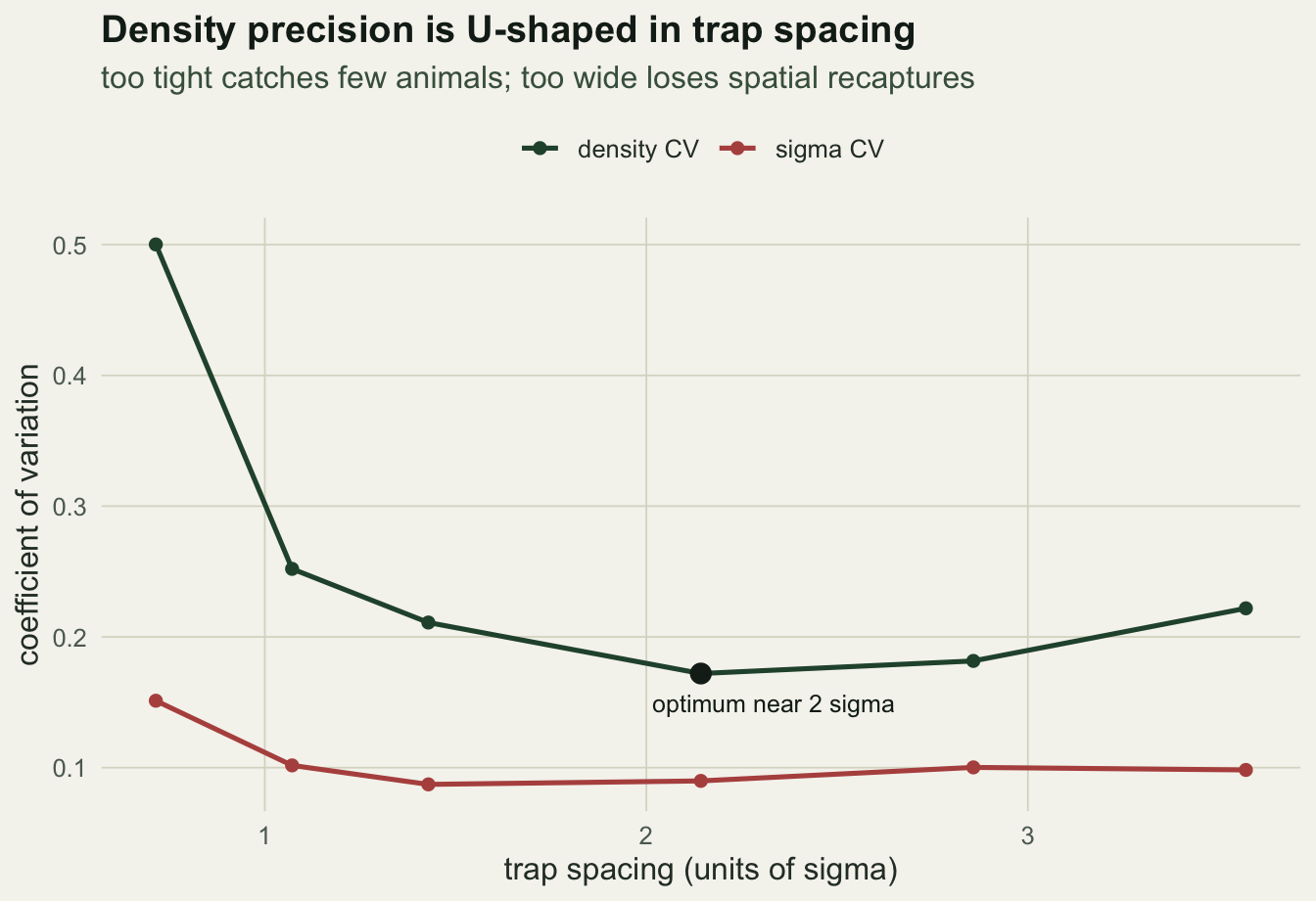
This post fixes the truth, sweeps the trap spacing across a range, and refits the from-scratch SCR likelihood many times at each spacing to measure the sampling variability of the density estimate. The result is a broad valley whose floor lies near two sigma, and a clear mechanism behind it.
## Spatial recaptures are the currency
The frequentist post leaned on spatial recaptures, animals caught at two or more traps, to pin down `sigma`. A capture at a single trap says an animal was nearby, but not how far it typically ranges. The number of spatial recaptures depends on the geometry. With a fixed budget of traps, tight spacing covers a small area (few animals enter it) while each caught animal hits many traps (many recaptures); wide spacing covers a large area (many animals) but each animal usually touches one trap (few recaptures). Density precision has to trade these off.
```{r}
#| label: setup
#| code-fold: true
#| code-summary: "Setup: packages, colours and plot theme"
#| results: hide
#| message: false
#| warning: false
library(ggplot2); library(tidyr)
paper <- "#f5f4ee"; ink <- "#16241d"; body <- "#2c3a31"; forest <- "#275139"
labelc <- "#46604a"; sage <- "#93a87f"; linec <- "#dad9ca"; faint <- "#5d6b61"
gold <- "#c9b458"; rust <- "#b5534e"
theme_te <- function(base_size = 12) {
  theme_minimal(base_size = base_size) +
    theme(
      plot.background  = element_rect(fill = paper, colour = NA),
      panel.background = element_rect(fill = paper, colour = NA),
      panel.grid.minor = element_blank(),
      panel.grid.major = element_line(colour = linec, linewidth = 0.3),
      axis.title = element_text(colour = body), axis.text = element_text(colour = faint),
      plot.title = element_text(colour = ink, face = "bold"),
      plot.subtitle = element_text(colour = labelc),
      legend.title = element_text(colour = body), legend.text = element_text(colour = body),
      strip.text = element_text(colour = ink, face = "bold")
    )
}
```
## One fit, then a sweep
The fitting function simulates a study at a given spacing (a 5 by 5 trap grid, a buffered state-space, activity centres from a Poisson process) and maximises the same integrated likelihood used in the basics post. It returns the density and `sigma` estimates plus the spatial-recapture count.
```{r}
#| label: fit-one
D_true <- 0.5; g0_true <- 0.30; sig_true <- 0.70; K <- 6

fit_one <- function(spacing) {
  tr    <- seq(0, 4 * spacing, by = spacing)          # 5 x 5 = 25 traps
  traps <- as.matrix(expand.grid(x = tr, y = tr)); J <- nrow(traps)
  buf   <- 4 * sig_true
  xl <- range(traps[, 1]) + c(-buf, buf); yl <- range(traps[, 2]) + c(-buf, buf)
  A  <- diff(xl) * diff(yl)
  N  <- rpois(1, D_true * A)
  sx <- runif(N, xl[1], xl[2]); sy <- runif(N, yl[1], yl[2])
  d2 <- outer(sx, traps[, 1], "-")^2 + outer(sy, traps[, 2], "-")^2
  Yf <- matrix(rbinom(N * J, K, g0_true * exp(-d2 / (2 * sig_true^2))), N, J)
  cc <- rowSums(Yf) > 0; Y <- Yf[cc, , drop = FALSE]; n <- nrow(Y)
  sr <- sum(rowSums(Y > 0) >= 2)
  rr <- sum(Y) - n                                     # recaptures: detections after the first
  if (n < 3) return(list(D = NA, sigma = NA, sr = sr, n = n, r = rr, ok = FALSE))

  hx <- diff(xl) / 26; hy <- diff(yl) / 26           # 26 x 26 equal cells
  gx <- seq(xl[1] + hx / 2, xl[2] - hx / 2, length.out = 26)   # cell centres
  gy <- seq(yl[1] + hy / 2, yl[2] - hy / 2, length.out = 26)
  G  <- as.matrix(expand.grid(x = gx, y = gy))
  d2G <- outer(G[, 1], traps[, 1], "-")^2 + outer(G[, 2], traps[, 2], "-")^2
  Cc  <- rowSums(lchoose(K, Y))
  negll <- function(th) {                             # same likelihood as the basics post
    Dd <- exp(th[1]); g0 <- plogis(th[2]); sg <- exp(th[3])
    P  <- g0 * exp(-d2G / (2 * sg^2))
    pb <- mean(1 - exp(rowSums(K * log1p(-P))))
    if (pb <= 0) return(1e10)
    LM <- Y %*% t(log(P)) + (K - Y) %*% t(log1p(-P)) + Cc
    m  <- apply(LM, 1, max); lf <- m + log(rowMeans(exp(LM - m)))
    -(dpois(n, Dd * A * pb, log = TRUE) + sum(lf) - n * log(pb))
  }
  st <- c(log(max(n, 1) / (A * 0.4)), qlogis(0.25), log(sig_true))
  ft <- tryCatch(optim(st, negll, method = "BFGS",
                       control = list(maxit = 400, reltol = 1e-9)), error = function(e) NULL)
  if (is.null(ft) || ft$convergence != 0) return(list(D = NA, sigma = NA, sr = sr, n = n, r = rr, ok = FALSE))
  Dh <- exp(ft$par[1]); sh <- exp(ft$par[3])
  list(D = Dh, sigma = sh, sr = sr, n = n, r = rr,
       ok = is.finite(Dh) && is.finite(sh) && sh < 4 * sig_true && Dh < 5 * D_true)
}
```
Now sweep the spacing from well under `sigma` to several times `sigma`, with many replicate studies at each, and summarise the coefficient of variation of the density estimate.
```{r}
#| label: sweep
set.seed(129)
spacings <- c(0.5, 0.75, 1.0, 1.5, 2.0, 2.5)
R <- 80
res <- data.frame()
for (sp in spacings) {
  Ds <- Ss <- SRs <- Ns <- RRs <- oks <- numeric(R)
  for (r in 1:R) { o <- fit_one(sp); Ds[r] <- o$D; Ss[r] <- o$sigma
    SRs[r] <- o$sr; Ns[r] <- o$n; RRs[r] <- o$r; oks[r] <- o$ok }
  use <- oks == 1
  res <- rbind(res, data.frame(
    spacing = sp, sigma_ratio = sp / sig_true,
    n_mean = mean(Ns), r_mean = mean(RRs), sr_frac = mean(SRs / pmax(Ns, 1)), usable = mean(use),
    D_cv = sd(Ds[use]) / mean(Ds[use]), sig_cv = sd(Ss[use]) / mean(Ss[use]),
    D_sig_cor = cor(Ds[use], Ss[use])))
}
best <- res$spacing[which.min(res$D_cv)]
```
The precision curve is U-shaped. At the tightest spacing (`r round(res$sigma_ratio[1], 2)` sigma) the array is small and only about `r round(res$n_mean[1])` animals are caught, so the density estimate has a coefficient of variation of `r round(res$D_cv[1], 2)`: high, despite a healthy spatial-recapture fraction of `r round(res$sr_frac[1], 2)`. At the widest spacing (`r round(res$sigma_ratio[6], 2)` sigma) about `r round(res$n_mean[6])` animals are caught, but the spatial-recapture fraction has collapsed to `r round(res$sr_frac[6], 2)`, a few fits fail (a usable fraction of `r round(res$usable[6], 2)`), although among the fits that work the sigma CV is `r round(res$sig_cv[6], 2)`, close to the `r round(res$sig_cv[which.min(res$D_cv)], 2)` at the optimum, and the density coefficient of variation climbs back to `r round(res$D_cv[6], 2)`. The minimum sits at a spacing of `r best` units, or `r round(best / sig_true, 2)` sigma, with a coefficient of variation of `r round(min(res$D_cv), 2)`, although with `r R` replicates per spacing the next spacing up is within Monte Carlo error of it, so the floor of the valley is located only roughly. That matches the standard guidance that traps should sit no more than about two sigma apart (Sun, Fuller and Royle 2014).
```{r}
#| label: fig-cv
#| fig-cap: "Coefficient of variation of the density estimate (and of sigma) against trap spacing in units of sigma, over many replicate studies at fixed trap number. Density precision is worst at the tightest spacing, best near two sigma, marked by the point, and slips again at wider spacings."
#| fig-alt: "Two lines against trap spacing in sigma units: the density CV falls steeply from the tightest spacing to its low point near two sigma and rises gently beyond it, and the sigma CV is highest at the tightest spacing and nearly flat elsewhere; a dot marks the density minimum."
#| fig-width: 7
#| fig-height: 4.8
cvl <- pivot_longer(res, c(D_cv, sig_cv), names_to = "which", values_to = "cv")
cvl$which <- factor(cvl$which, c("D_cv", "sig_cv"), c("density CV", "sigma CV"))
bmin <- res[which.min(res$D_cv), ]
p1 <- ggplot(cvl, aes(sigma_ratio, cv, colour = which)) +
  geom_line(linewidth = 0.9) + geom_point(size = 1.8) +
  geom_point(data = bmin, aes(sigma_ratio, D_cv), colour = ink, size = 3.2, inherit.aes = FALSE) +
  annotate("text", x = bmin$sigma_ratio, y = bmin$D_cv, label = "optimum near 2 sigma",
           vjust = 2.2, hjust = 0.2, colour = ink, size = 3.3) +
  scale_colour_manual(values = c("density CV" = forest, "sigma CV" = rust), name = NULL) +
  labs(x = "trap spacing (units of sigma)", y = "coefficient of variation",
       title = "Density precision is U-shaped in trap spacing",
       subtitle = "too tight catches few animals; too wide loses spatial recaptures") +
  theme_te() + theme(legend.position = "top")
p1
```
## The two forces behind the U
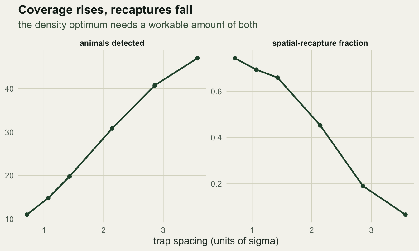
Splitting the drivers makes the trade-off explicit. As spacing widens, the number of animals detected rises steadily (more ground covered), while the fraction of animals recaptured at a second trap falls just as steadily (traps too far apart to both catch the same animal). Density precision needs both: enough animals for a stable count, and enough spatial recaptures. At the widest spacing, where recaptures are rare, the `sigma` estimate itself stayed about as precise as at the optimum, but the density estimate became more strongly tied to it: the correlation between the two estimates was `r round(res$D_sig_cor[6], 2)` there, against `r round(res$D_sig_cor[which.min(res$D_cv)], 2)` at the optimum. The optimum is where the two curves cross usefully, not where either is maximised.
```{r}
#| label: fig-drivers
#| fig-cap: "The two competing quantities against trap spacing: animals detected (rising with area) and the spatial-recapture fraction (falling as traps spread apart). The density optimum needs a workable amount of both, so it falls between the extremes rather than at either end."
#| fig-alt: "Two panels against trap spacing in sigma units: animals detected rises from about ten to fifty, while the spatial-recapture fraction falls from about three-quarters to near zero."
#| fig-width: 7
#| fig-height: 4.2
dl <- pivot_longer(res, c(n_mean, sr_frac), names_to = "metric", values_to = "value")
dl$metric <- factor(dl$metric, c("n_mean", "sr_frac"),
                    c("animals detected", "spatial-recapture fraction"))
p2 <- ggplot(dl, aes(sigma_ratio, value)) +
  geom_line(colour = forest, linewidth = 0.9) + geom_point(colour = forest, size = 1.8) +
  facet_wrap(~ metric, scales = "free_y") +
  labs(x = "trap spacing (units of sigma)", y = NULL,
       title = "Coverage rises, recaptures fall",
       subtitle = "the density optimum needs a workable amount of both") +
  theme_te()
p2
```
## A rule of thumb, checked against the sweep
Efford and Boulanger (2019) give a shortcut that avoids the simulation: the relative standard error of the density estimate is close to $1/\sqrt{\min(n, r)}$, where $n$ is the number of animals detected and $r$ the number of recaptures, every detection of an animal after its first. The `secrdesign` documentation calls the result approximate, notes that it disregards possible bias, suggests multiplying it by a correction factor of about 1.2 for a hollow grid and 1.4 for a line of detectors, and advises checking it with a few simulations. The sweep above is that check for a full five by five grid, so the rule can be set against the realised coefficient of variation spacing by spacing.
```{r rule}
res$rule <- 1 / sqrt(pmin(res$n_mean, res$r_mean))
res$cv_over_rule <- res$D_cv / res$rule
hr95_diam <- 2 * sqrt(qchisq(0.95, 2)) * sig_true   # 95 per cent home range, bivariate normal
array_w <- 4 * spacings
stopifnot(res$n_mean[4] < res$r_mean[4], res$n_mean[5] > res$r_mean[5],
          res$cv_over_rule[1] > 1.3, array_w[1] < hr95_diam)
print(round(res[, c("sigma_ratio", "n_mean", "r_mean", "rule", "D_cv", "cv_over_rule")], 3))
print(round(c(home_range_95_diameter = hr95_diam, tightest_array_width = array_w[1]), 3))
```
From `r round(res$sigma_ratio[2], 2)` sigma upwards the rule and the simulation agree closely: the realised coefficient of variation is between `r sprintf("%.2f", min(res$cv_over_rule[-1]))` and `r sprintf("%.2f", max(res$cv_over_rule[-1]))` times the rule. The rule also explains the shape of the valley. At tight spacings recaptures are plentiful and the number of animals is the smaller count, so precision is limited by $n$; at wide spacings the recaptures run short and $r$ takes over. The two counts cross between `r round(res$sigma_ratio[4], 2)` and `r round(res$sigma_ratio[5], 2)` sigma, which is where the floor of the valley lies.
The rule fails at the tightest spacing. There it predicts `r sprintf("%.2f", res$rule[1])` and the simulation gives `r sprintf("%.2f", res$D_cv[1])`, `r sprintf("%.2f", res$cv_over_rule[1])` times as much. The whole array is `r sprintf("%.1f", array_w[1])` units wide, less than the `r sprintf("%.1f", hr95_diam)` unit diameter of an animal's 95 per cent home range, so the array sees only part of the range of each animal it catches and says little about how far that range extends. That is one of the cases the `secrdesign` documentation lists as outside the rule, an array much smaller than a home range.
Two limits sit outside this sweep. The rule is about precision only, so a design that gives a biased estimate, for instance through detection that differs between the sexes, can look as good on it as one that does not. And it assumes that activity centres are placed independently. Efford and Fletcher (2025) show that when animals cluster, or the density surface itself varies from one realisation to the next, confidence intervals for density cover the truth much less often than they should, and that a reliable correction needs either knowledge of the process that generated the clustering or independent replicate arrays. A group-living species is a reason to simulate rather than to trust the shortcut.
```{r}
#| label: thumb
#| include: false
ggsave("thumbnail.png", p1 + labs(title = NULL, subtitle = NULL) +
theme(legend.position = "none"),
width = 7.5, height = 5.4, dpi = 100, bg = paper)
```
## Takeaways
The precision of an SCR density estimate is a design choice, not a given. Trap spacing relative to `sigma` sets it: too tight and the array is too small to catch many animals, too wide and spatial recaptures become rare, with density uncertainty rising at both ends (although in this sweep the `sigma` estimate itself stayed about as precise at the widest spacing as at the optimum, among the fits that worked). For a fixed number of traps the sweet spot here is near two sigma, in line with the published recommendation. The shortcut $1/\sqrt{\min(n, r)}$ follows the simulated precision closely except where the array is narrower than a home range, and it says nothing about bias or about animals that cluster. The practical implication is that you cannot plan an SCR study without a working guess at `sigma` (from a pilot, similar species, or telemetry), because the whole design hinges on it. The next post keeps the design fixed and turns to the detection process itself: covariates on `g0`, and how to check whether the fitted detection model actually fits.
## References
Sun, C. C., Fuller, A. K. and Royle, J. A. 2014. PLoS ONE 9(2):e88025 (10.1371/journal.pone.0088025).
Efford, M. 2004. Oikos 106(3):598-610 (10.1111/j.0030-1299.2004.13043.x).
Borchers, D. L. and Efford, M. G. 2008. Biometrics 64(2):377-385 (10.1111/j.1541-0420.2007.00927.x).
Wilton, C. M., Puckett, E. E., Beringer, J., Gardner, B., Eggert, L. S. and Belant, J. L. 2014. PLoS ONE 9(10):e111257 (10.1371/journal.pone.0111257).
Royle, J. A., Chandler, R. B., Sollmann, R. and Gardner, B. 2014. Spatial Capture-Recapture. Academic Press (ISBN 978-0-12-405939-9).
Efford, M. G. and Boulanger, J. 2019. Methods in Ecology and Evolution 10(9):1529-1535 (10.1111/2041-210X.13239).
Efford, M. G. and Fletcher, D. 2025. Peer Community Journal 5:e70 (10.24072/pcjournal.578).
## Related tutorials
- [Spatial capture-recapture from scratch](../spatial-capture-recapture-basics/)
- [Detection covariates and checking in SCR](../scr-detection-covariates/)
- [Trap-specific responses in spatial capture-recapture](../trap-specific-responses-in-scr/)
- [Spatial capture-recapture on a meandering stream](../spatial-capture-recapture-on-a-stream-network/)