library(ggplot2)
library(patchwork)

te_paper  <- "#f5f4ee"
te_ink    <- "#16241d"
te_body   <- "#2c3a31"
te_forest <- "#275139"
te_rust   <- "#b5534e"
te_gold   <- "#c9b458"
te_line   <- "#dad9ca"

theme_datasheet <- function() {
  theme_minimal(base_size = 12) +
    theme(plot.background  = element_rect(fill = te_paper, colour = NA),
          panel.background = element_rect(fill = te_paper, colour = NA),
          panel.grid.major = element_line(colour = te_line, linewidth = 0.3),
          panel.grid.minor = element_blank(),
          text             = element_text(colour = te_body),
          plot.title       = element_text(colour = te_ink, face = "bold"),
          plot.subtitle    = element_text(colour = te_body),
          axis.text        = element_text(colour = te_body))
}Trap-specific responses in spatial capture-recapture
R
capture-recapture
spatial
behavioural response
simulation
ecology tutorial
When animals learn one baited trap, spatial capture-recapture in R reads the pile-up of recaptures as a short sigma. A global Mb cannot fix it; Mbk can.
A small-mammal grid of 49 baited hair tubes runs for six nights, and the hairs left on the sticky patch inside each tube are genotyped, so each genotyped sample is a detection of a known animal. A wood mouse that leaves hair in tube C4 on the first night has found oats there, and on the nights that follow it turns up in C4 again, and again, while the tubes one row over, which sit just as close to where it lives, rarely record it. Nothing about the mouse’s home range has changed. What has changed is that one tube is now worth visiting and the others are not.
Spatial capture-recapture reads the spread of an animal’s captures across the grid as information about how far it ranges. Spatial capture-recapture from scratch builds the likelihood that does this, with a half-normal detection function whose scale sigma is estimated from where each animal was caught, and SCR sampling design and precision puts the point bluntly: “A capture at a single trap says an animal was nearby, but not how far it typically ranges.” A mouse that keeps returning to C4 is a pile of captures at a single trap (a detection at a hair tube counts as a capture here). The model has no way to know the pile is about bait, so it reads it as a mouse that does not range far.
The standard answer to a trap response is model Mb, which Royle, Chandler, Sollmann and Gardner (2014) carry into spatial models in their chapter on variation in encounter probability. It works on this site. Capture heterogeneity: Mt, Mb and Mh in R generates trap-shy data and fits a global Mb, in which capture probability changes once and everywhere after the first capture, and Mb is the one model whose estimate sits on the truth. The capture-heterogeneity post fits a trap response that has no address, and there the global model is the repair; on a grid, a global term can change how often an animal is caught but not where, and sigma stays short until the model knows which trap the animal learned. The secr package calls the trap-specific version bk, an animal by site learned response, and Schmidt, Graves, Pederson and Carroll (2022) met it in black bear hair corrals baited with a scent lure, where a trap-specific behavioural term was strongly supported at one of their study areas, and a behavioural term in the detection model raised density estimates relative to models without one. Schmidt and colleagues also fitted a model without the behavioural term to data simulated with it; their main text reports only the matched fits, and I have not seen the mismatched results in their appendix, so this post makes no claim about priority. It measures what ignoring the local response does to sigma in a controlled setting.
Two other posts mark the edges. Detection covariates and checking in SCR lets baseline detection differ between traps because some “use more attractive lures”, which is a fixed property of the trap shared by every animal; here the attraction belongs to one animal and one trap and switches on only after a capture. Disturbed animals in repeated counts is the same idea with no marks at all: a counted animal is detected afterwards with a different probability, and a count-only version of Mb repairs the N-mixture estimate. This post adds the address.
Where the later captures fall
The design is a 7 by 7 grid of proximity detectors run for six occasions, with the half-normal detection shape of Efford (2004) and sigma of 0.8 units. Proximity detectors let an animal be recorded at several traps on one occasion, as hair tubes and cameras do; live traps do not, and that case is not simulated (Honest limits). Activity centres are uniform over the grid plus a buffer of four sigma. At the base spacing of one unit, which is 1.25 sigma, the state space holds 150 animals, and that density is held fixed at every spacing used later, so a wider grid sits in a larger state space with proportionally more animals. Naive detection at the activity centre is 0.10.
Three truths share that design. With no response, detection never changes. With a global response, an animal’s detection at every trap rises after its first capture anywhere. With a trap-specific response, detection rises only at a trap where that animal has already been caught, and stays at the naive value at every other trap.
sigma_true <- 0.8                      # detection scale, grid units
n_side     <- 7                        # 7 x 7 proximity detectors
k_occ      <- 6                        # occasions
buffer     <- 4 * sigma_true           # state space beyond the outer traps
cell_target <- 0.6                     # mask cell size, grid units
p0_naive   <- 0.10                     # detection at the centre before capture
density_fix <- 150 / (6 + 2 * buffer)^2  # animals per unit area, held fixed

make_design <- function(spacing_sigma) {
  spacing <- spacing_sigma * sigma_true
  g   <- (0:(n_side - 1)) * spacing
  tr  <- as.matrix(expand.grid(x = g, y = g))
  lo  <- -buffer; hi <- max(g) + buffer
  n_cell <- round((hi - lo) / cell_target)
  mg  <- seq(lo, hi, length.out = n_cell + 1)
  mg  <- (mg[-1] + mg[-length(mg)]) / 2
  msk <- as.matrix(expand.grid(x = mg, y = mg))
  d2  <- outer(msk[, 1], tr[, 1], "-")^2 + outer(msk[, 2], tr[, 2], "-")^2
  list(tr = tr, d2 = d2, lo = lo, hi = hi, spacing = spacing,
       cell = (hi - lo) / n_cell, n_true = round(density_fix * (hi - lo)^2))
}

# one capture history array (animals x traps x occasions) for detected animals
simulate_caps <- function(des, p0, p0_after, response) {
  n_all <- des$n_true; n_tr <- nrow(des$tr)
  sx <- runif(n_all, des$lo, des$hi); sy <- runif(n_all, des$lo, des$hi)
  h  <- exp(-(outer(sx, des$tr[, 1], "-")^2 + outer(sy, des$tr[, 2], "-")^2) /
              (2 * sigma_true^2))
  at_trap <- matrix(FALSE, n_all, n_tr); any_trap <- rep(FALSE, n_all)
  y <- array(FALSE, c(n_all, n_tr, k_occ))
  for (k in seq_len(k_occ)) {
    resp <- switch(response,
                   local  = at_trap,
                   global = matrix(any_trap, n_all, n_tr),
                   none   = matrix(FALSE, n_all, n_tr))
    yk <- matrix(runif(n_all * n_tr) < ifelse(resp, p0_after, p0) * h, n_all, n_tr)
    y[, , k] <- yk
    at_trap  <- at_trap | yk
    any_trap <- any_trap | rowSums(yk) > 0
  }
  y[apply(y, 1, any), , , drop = FALSE]
}
des_base <- make_design(1.25)
The mask cell comes out at 0.590 units at the base spacing. The first thing to look at is the raw data, before any model: for every detected animal, where do its captures after the first occasion fall, measured from the trap where it was first caught? The response in this check is fourfold, detection 0.10 before and 0.40 after.
set.seed(2716)
n_pile <- 100
later_dist <- function(y, des) {
  out <- numeric(0)
  for (i in seq_len(dim(y)[1])) {
    yi <- y[i, , ]
    k1 <- which(colSums(yi) > 0)[1]
    j1 <- which(yi[, k1])[1]
    if (k1 == k_occ) next
    hits <- which(yi[, (k1 + 1):k_occ, drop = FALSE], arr.ind = TRUE)[, 1]
    out <- c(out, sqrt(colSums((t(des$tr[hits, , drop = FALSE]) - des$tr[j1, ])^2)) /
                  des$spacing)
  }
  out
}
pile_one <- function(response) {
  d <- unlist(lapply(seq_len(n_pile), function(r)
    later_dist(simulate_caps(des_base, p0_naive, 0.40, response), des_base)))
  cls <- cut(d, c(-0.01, 0.5, 1.2, 1.5, 2.1, Inf),
             labels = c("same trap", "1", "1.41", "2", "more than 2"))
  data.frame(response = response, dist = levels(cls),
             share = as.vector(table(cls)) / length(d), n_later = length(d))
}
pile <- do.call(rbind, lapply(c("none", "global", "local"), pile_one))
same_share <- setNames(pile$share[pile$dist == "same trap"],
                       pile$response[pile$dist == "same trap"])
n_later_all <- setNames(pile$n_later[pile$dist == "same trap"],
pile$response[pile$dist == "same trap"])pile$dist <- factor(pile$dist, levels = c("same trap", "1", "1.41", "2", "more than 2"))
pile$response <- factor(pile$response, levels = c("none", "global", "local"),
labels = c("no response", "global response", "trap-specific response"))
ggplot(pile, aes(dist, share, fill = response)) +
geom_col(position = position_dodge(width = 0.8), width = 0.75) +
scale_fill_manual(values = c(te_gold, te_forest, te_rust), name = NULL) +
labs(x = "distance from first-capture trap (trap spacings)",
y = "share of later captures",
title = "A learned trap collects the later captures") +
theme_datasheet() +
theme(legend.position = "top")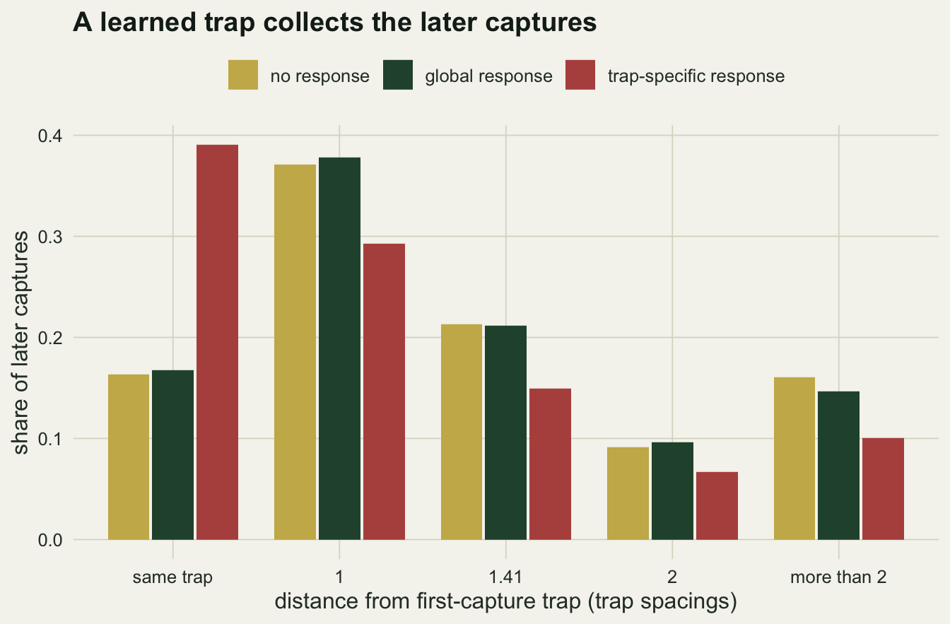
With no response, 16 per cent of later captures land back in the first-capture trap, a share set by the grid geometry alone. A global response leaves that share at 17 per cent: the animals are caught more often, 21361 later captures against 5318 over the same number of data sets, but they are caught in the same places. A trap-specific response moves the share to 39 per cent, and every other distance class loses what the first trap gains. That tighter spatial pattern is what a half-normal detection function will fit.
Three models on one likelihood
The likelihood is the conditional one of Borchers and Efford (2008): each detected animal’s capture history is integrated over a discrete mask of possible activity centres, and the product is divided by the probability of being detected at all, raised to the number detected. Abundance in the state space then follows as a Horvitz-Thompson estimate, the number detected divided by the mean detection probability over the mask. The three models differ only in which occasions count as “after the response” for each animal and trap: none of them in M0, every occasion after the animal’s first capture in the global Mb, and every occasion after the animal’s first capture at that particular trap in the trap-specific model, called Mbk here. The probability of being detected at all involves only naive detection in all three, because nothing has been learned before a first capture.
The code builds three tallies per animal and trap (naive captures, responded captures, responded occasions) so that the log likelihood on the mask is a few sums over the traps where each animal was caught.
tallies <- function(y, model) {
  n <- dim(y)[1]; n_tr <- dim(y)[2]
  n1 <- m1 <- b <- matrix(0, n_tr, n)
  seen_here <- matrix(FALSE, n, n_tr); seen_any <- rep(FALSE, n)
  for (k in seq_len(k_occ)) {
    yk <- y[, , k]
    resp <- switch(model,
                   M0  = matrix(FALSE, n, n_tr),
                   Mb  = matrix(seen_any, n, n_tr),
                   Mbk = seen_here)
    n1 <- n1 + t(yk & !resp)       # captures while naive
    m1 <- m1 + t(yk & resp)        # captures after the response
    b  <- b + t(resp)              # occasions after the response
    seen_here <- seen_here | yk
    seen_any  <- seen_any | rowSums(yk) > 0
  }
  list(n1 = n1, m1 = m1, b = b)
}

# the tallies are sparse: only traps where an animal was caught carry counts,
# so each product with a mask x trap matrix is a sum over those traps alone
to_triplet <- function(tab) {
  w <- which(tab != 0, arr.ind = TRUE)
  list(j = w[, 1], i = w[, 2], v = tab[w], n = ncol(tab))
}
sparse_prod <- function(lmat, trip) {
  out <- matrix(0, nrow(lmat), trip$n)
  if (length(trip$v) == 0) return(out)
  r <- rowsum(t(lmat[, trip$j, drop = FALSE]) * trip$v, trip$i)
  out[, as.integer(rownames(r))] <- t(r)
  out
}

fit_scr <- function(y, des, model, start = NULL) {
  tl <- tallies(y, model); n <- dim(y)[1]
  s_n1 <- to_triplet(tl$n1); s_m1 <- to_triplet(tl$m1)
  if (model == "Mb") b_animal <- tl$b[1, ] else s_b <- to_triplet(tl$b)
  nll <- function(th) {
    p0 <- plogis(th[1]); sg <- exp(th[2])
    p0_after <- if (model == "M0") p0 else plogis(th[3])
    h  <- exp(-des$d2 / (2 * sg^2))
    pr <- pmin(p0 * h, 1 - 1e-12); pr_after <- pmin(p0_after * h, 1 - 1e-12)
    l0 <- log1p(-pr); l0_after <- log1p(-pr_after)
    lf <- sparse_prod(log(pr) - l0, s_n1) + k_occ * rowSums(l0)
    if (model != "M0") {
      lf <- lf + sparse_prod(log(pr_after) - l0_after, s_m1)
      # under Mb the responded occasions are the same at every trap
      lf <- lf + if (model == "Mb") outer(rowSums(l0_after - l0), b_animal) else
        sparse_prod(l0_after - l0, s_b)
    }
    pdot <- 1 - exp(k_occ * rowSums(l0))
    mx <- lf[cbind(max.col(t(lf), ties.method = "first"), seq_len(n))]
    v  <- -(sum(mx + log(colSums(exp(lf - rep(mx, each = nrow(lf)))))) - n * log(sum(pdot)))
    if (is.finite(v)) v else 1e10
  }
  st <- if (is.null(start)) c(qlogis(0.1), log(1)) else start
  o  <- optim(st, nll, method = "BFGS", control = list(maxit = 500))
  p0 <- plogis(o$par[1]); sg <- exp(o$par[2])
  pdot <- 1 - exp(k_occ * rowSums(log1p(-pmin(p0 * exp(-des$d2 / (2 * sg^2)), 1 - 1e-12))))
  list(par = o$par, p0 = p0, sigma = sg,
       p0_after = if (model == "M0") p0 else plogis(o$par[3]),
       n_hat = n / mean(pdot), aic = 2 * o$value + 2 * length(o$par),
       conv = o$convergence)
}

fit_three <- function(y, des) {
  f0 <- fit_scr(y, des, "M0")
  st <- c(f0$par, f0$par[1])          # Mb and Mbk start from the M0 answer
  list(M0 = f0, Mb = fit_scr(y, des, "Mb", st), Mbk = fit_scr(y, des, "Mbk", st))
}

set.seed(4417)
y_ex <- simulate_caps(des_base, p0_naive, 0.40, "local")
fits_ex <- fit_three(y_ex, des_base)
ex_tab <- data.frame(model = names(fits_ex),
  sigma_ratio = sapply(fits_ex, function(f) f$sigma / sigma_true),
  p0 = sapply(fits_ex, `[[`, "p0"), p0_after = sapply(fits_ex, `[[`, "p0_after"),
  aic = sapply(fits_ex, `[[`, "aic"))
ex_tab$d_aic <- ex_tab$aic - min(ex_tab$aic)
print(ex_tab[, c("model", "sigma_ratio", "p0", "p0_after", "d_aic")], digits = 3, row.names = FALSE)
model sigma_ratio p0 p0_after d_aic
M0 0.881 0.207 0.207 33.0
Mb 0.881 0.116 0.244 22.5
Mbk 1.019 0.115 0.383 0.0One data set from the fourfold trap-specific truth catches 59 of the 150 animals. M0 puts sigma at 0.88 of its true value. The global Mb estimates detection after capture at 0.244 against 0.116 before, so it has found the response, and it still puts sigma at 0.88. The trap-specific model estimates 0.383 after and 0.115 before, puts sigma at 1.02, and is ahead of Mb by 22.5 AIC units. One data set is an anecdote; the next section repeats it.
Sigma shrinks, and the global term cannot move it
Four settings share the base spacing of 1.25 sigma. Two are trap-happy trap-specific responses, twofold (detection 0.10 to 0.20) and fourfold (0.10 to 0.40). One is trap-shy and trap-specific, halving detection from 0.30 to 0.15. The fourth is the control: a fourfold response that is global, so the truth is Mb. All design constants except the number of draws in the fourfold trap-specific cells at 1.25 and 2.0 sigma were fixed before any fits were run. The twofold and fourfold trap-specific cells get 40 simulated data sets each, the global control 20 and the trap-shy cell 10.
one_draw <- function(des, p0, p0_after, response) {
  y  <- simulate_caps(des, p0, p0_after, response)
  f  <- fit_three(y, des)
  traps_per <- mean(rowSums(apply(y, c(1, 2), any)))
  c(n_caught = dim(y)[1], traps = traps_per,
    s_M0 = f$M0$sigma, s_Mb = f$Mb$sigma, s_Mbk = f$Mbk$sigma,
    N_M0 = f$M0$n_hat, N_Mb = f$Mb$n_hat, N_Mbk = f$Mbk$n_hat,
    best = which.min(c(f$M0$aic, f$Mb$aic, f$Mbk$aic)),
    conv = f$M0$conv + f$Mb$conv + f$Mbk$conv)
}
run_cell <- function(id, spacing_sigma, p0, p0_after, response, n_draw) {
  des <- make_design(spacing_sigma)
  m <- t(replicate(n_draw, one_draw(des, p0, p0_after, response)))
  data.frame(cell = id, spacing_sigma = spacing_sigma, ratio = p0_after / p0,
             response = response, n_true = des$n_true, m)
}
t_cells <- proc.time()
set.seed(8203)
cells <- rbind(
  run_cell("A", 1.25, 0.10, 0.20, "local",  40),
  run_cell("B", 1.25, 0.10, 0.40, "local",  40),
  run_cell("E", 1.25, 0.10, 0.40, "global", 20),
  run_cell("F", 1.25, 0.30, 0.15, "local",  10),
  run_cell("C", 2.00, 0.10, 0.40, "local",  40),
  run_cell("D", 2.50, 0.10, 0.40, "local",  20))
t_cells <- (proc.time() - t_cells)[["user.self"]]
for (m in c("M0", "Mb", "Mbk")) {
  cells[[paste0("sr_", m)]] <- cells[[paste0("s_", m)]] / sigma_true
  cells[[paste0("nr_", m)]] <- cells[[paste0("N_", m)]] / cells$n_true
}
cell_sum <- do.call(rbind, lapply(split(cells, cells$cell), function(d) {
  data.frame(cell = d$cell[1], draws = nrow(d), n_true = d$n_true[1],
    n_caught = median(d$n_caught),
    traps = mean(d$traps),
    sr_M0 = median(d$sr_M0), sr_Mb = median(d$sr_Mb), sr_Mbk = median(d$sr_Mbk),
    mean_Mb = mean(d$sr_Mb), se_Mb = sd(d$sr_Mb) / sqrt(nrow(d)),
    lo_Mb = min(d$sr_Mb), hi_Mb = max(d$sr_Mb),
    lo_Mbk = min(d$sr_Mbk), hi_Mbk = max(d$sr_Mbk),
    gap = mean(d$sr_Mbk - d$sr_Mb), gap_se = sd(d$sr_Mbk - d$sr_Mb) / sqrt(nrow(d)),
    pick_M0 = mean(d$best == 1), pick_Mb = mean(d$best == 2), pick_Mbk = mean(d$best == 3),
    nr_M0 = median(d$nr_M0), nr_Mb = median(d$nr_Mb), nr_Mbk = median(d$nr_Mbk),
    nr_Mb_hi = max(d$nr_Mb), nr_Mb_n2 = sum(d$nr_Mb > 2), nr_Mbk_lo = min(d$nr_Mbk), nr_Mbk_hi = max(d$nr_Mbk),
    n_fail = sum(d$conv > 0))
}))
cs <- function(id, col) cell_sum[cell_sum$cell == id, col]
bc_diff <- cs("B", "mean_Mb") - cs("C", "mean_Mb")
bc_se   <- sqrt(cs("B", "se_Mb")^2 + cs("C", "se_Mb")^2)
print(cell_sum[, c("cell", "draws", "sr_M0", "sr_Mb", "sr_Mbk", "pick_Mbk")], digits = 3,
      row.names = FALSE)
cell draws sr_M0 sr_Mb sr_Mbk pick_Mbk
A 40 0.952 0.953 1.020 0.95
B 40 0.823 0.824 0.988 1.00
C 40 0.781 0.787 1.003 1.00
D 20 0.769 0.777 1.017 0.75
E 20 1.000 0.996 1.040 0.00
F 10 1.039 1.038 0.991 1.00sig_long <- do.call(rbind, lapply(c("M0", "Mb", "Mbk"), function(m)
data.frame(cell = cells$cell, model = m, ratio = cells[[paste0("sr_", m)]])))
sig_long <- sig_long[sig_long$cell %in% c("A", "B", "F", "E"), ]
cell_lab <- c(A = "trap-specific, twofold", B = "trap-specific, fourfold",
F = "trap-specific, trap-shy (half)", E = "control: global, fourfold")
sig_long$panel <- factor(cell_lab[sig_long$cell], levels = cell_lab)
sig_long$model <- factor(sig_long$model, levels = c("M0", "Mb", "Mbk"))
sig_med <- aggregate(ratio ~ panel + model, data = sig_long, FUN = median)
set.seed(11)
ggplot(sig_long, aes(model, ratio, colour = model)) +
geom_hline(yintercept = 1, linetype = "dashed", colour = te_ink, linewidth = 0.5) +
geom_jitter(width = 0.15, height = 0, size = 1.3, alpha = 0.6) +
geom_crossbar(data = sig_med, aes(ymin = ratio, ymax = ratio), width = 0.5,
linewidth = 0.6, colour = te_ink) +
scale_colour_manual(values = c(M0 = te_gold, Mb = te_forest, Mbk = te_rust), guide = "none") +
facet_wrap(~ panel, ncol = 2) +
labs(x = "model fitted", y = "estimated sigma / true sigma",
title = "Only the trap-specific model follows the address") +
theme_datasheet() +
theme(strip.text = element_text(colour = te_ink, face = "bold"))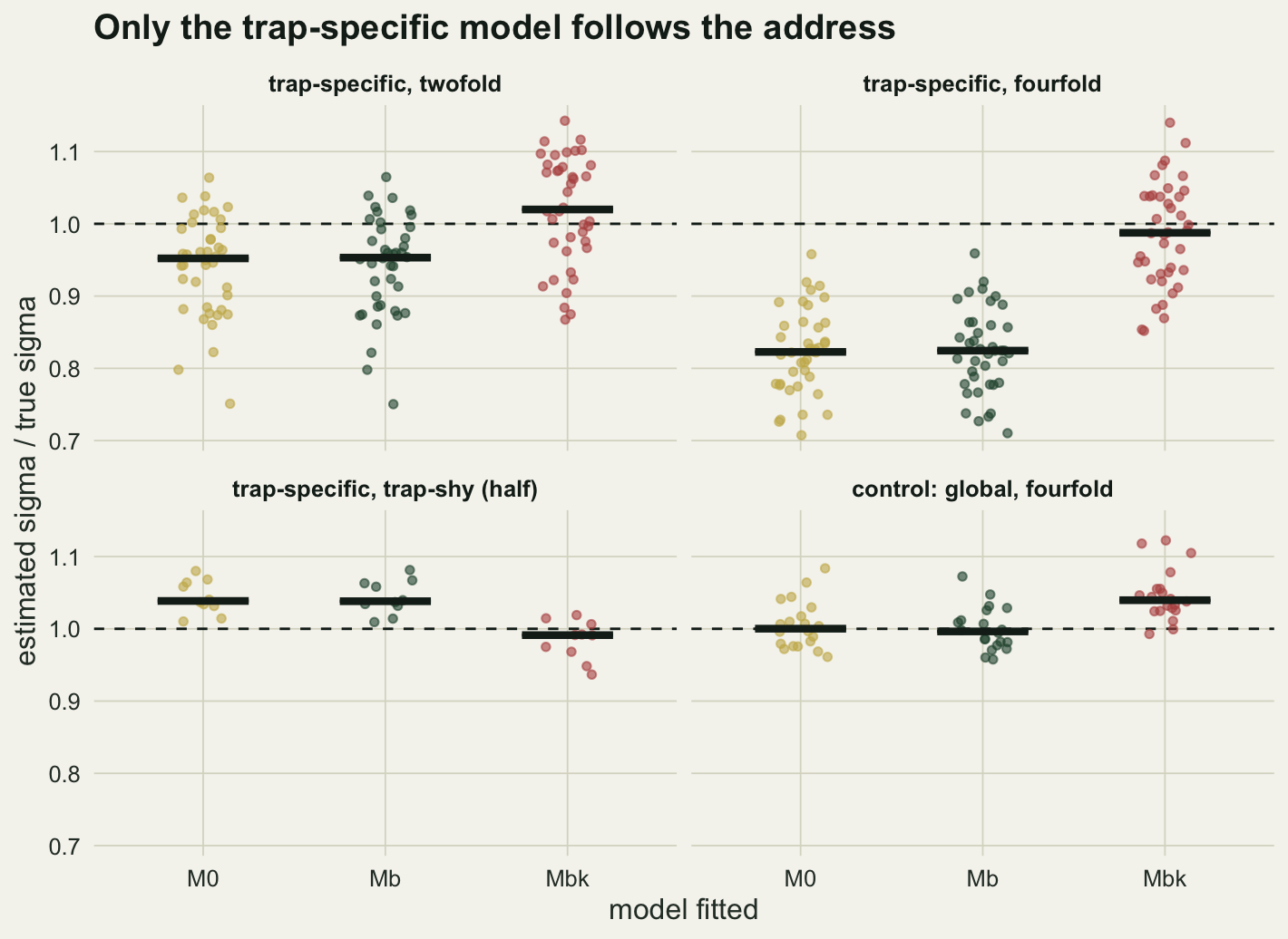
At the fourfold trap-happy response the median sigma is 0.82 of the truth under M0 and 0.82 under the global Mb, with Mb ranging from 0.71 to 0.96 over the 40 data sets. The global term leaves sigma where M0 put it. The trap-specific model gives 0.99, ranging from 0.85 to 1.14, and the mean paired difference between it and Mb on the same data is 0.161 (Monte Carlo standard error 0.005). AIC picks the trap-specific model in 100 per cent of the data sets.
The twofold response, close to the rise that Schmidt and colleagues took from their own bear data, does much less damage. M0 and Mb both give a median of 0.95 and the trap-specific model 1.02. The paired difference is 0.077 (standard error 0.005) over 40 data sets, so the direction is the same as at fourfold, but the shortfall under Mb is small against the spread of single estimates, which runs from 0.75 to 1.06. AIC still prefers the trap-specific model in 95 per cent of them.
The trap-shy cell runs the other way, as the mechanism says it should: halving detection at the learned trap pushes later captures off it, and M0 and Mb read the wider spread as a sigma of 1.04, while the trap-specific model gives 0.99. It is based on 10 data sets.
The control settles what the cause is. When the fourfold response is global, M0, which ignores the response altogether, still gets sigma right at 1.00, the correct Mb gives 1.00, and AIC picks Mb in 100 per cent of data sets. A response on its own does not bias sigma. A response with an address does. The trap-specific model fitted to the global truth gives 1.04, so it is not a free insurance policy either: fitting the wrong address pushes sigma the other way, although by less.
Wider spacing, larger damage
SCR sampling design and precision found its precision optimum near two sigma and quotes the standard guidance “that traps should sit no more than about two sigma apart (Sun, Fuller and Royle 2014)”. Two more cells run the fourfold trap-specific response at a spacing of 2.0 sigma, which is that guidance, and at 2.5 sigma, just past it, with density held at the base value so that the state space holds 250 and 330 animals.
sp_cells <- cell_sum[cell_sum$cell %in% c("B", "C", "D"), ]
sp_cells$spacing <- c(B = 1.25, C = 2.0, D = 2.5)[sp_cells$cell]
sp_long <- do.call(rbind, lapply(c("M0", "Mb", "Mbk"), function(m) {
  d <- cells[cells$cell %in% c("B", "C", "D"), ]
  r <- d[[paste0("sr_", m)]]
  data.frame(spacing = tapply(d$spacing_sigma, d$cell, `[`, 1), model = m,
             med = tapply(r, d$cell, median), lo = tapply(r, d$cell, min),
             hi = tapply(r, d$cell, max))
}))
sp_long$model <- factor(sp_long$model, levels = c("M0", "Mb", "Mbk"))
pos <- position_dodge(width = 0.18)
p_sig <- ggplot(sp_long, aes(spacing, med, colour = model, shape = model)) +
  geom_hline(yintercept = 1, linetype = "dashed", colour = te_ink, linewidth = 0.5) +
  geom_errorbar(aes(ymin = lo, ymax = hi), width = 0, linewidth = 0.6, position = pos) +
  geom_point(size = 2.6, position = pos) +
  scale_colour_manual(values = c(M0 = te_gold, Mb = te_forest, Mbk = te_rust), name = NULL) +
  scale_shape_manual(values = c(M0 = 16, Mb = 17, Mbk = 15), name = NULL) +
  scale_x_continuous(breaks = c(1.25, 2, 2.5)) +
  labs(x = "trap spacing (sigma units)", y = "estimated sigma / true sigma",
       title = "Spacing does not rescue Mb") +
  theme_datasheet() + theme(legend.position = "top")
p_tr <- ggplot(sp_cells, aes(spacing, traps)) +
  geom_line(colour = te_ink, linewidth = 0.6) +
  geom_point(colour = te_ink, size = 2.6) +
  scale_x_continuous(breaks = c(1.25, 2, 2.5)) +
  coord_cartesian(ylim = c(1, NA)) +
  labs(x = "trap spacing (sigma units)", y = "distinct traps per animal",
       title = "Spatial recaptures") +
  theme_datasheet()
(p_sig | p_tr) + plot_layout(widths = c(2, 1)) +
  plot_annotation(theme = theme_datasheet())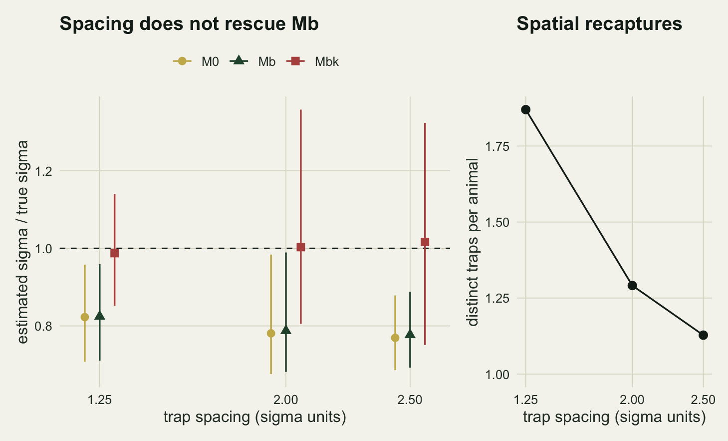
At 2.0 sigma the median sigma under Mb is 0.79, against 0.82 at 1.25 sigma, and at 2.5 sigma it is 0.78. The means tell the same story with a standard error attached: 0.824 (standard error 0.009) at 1.25 sigma and 0.790 (0.009) at 2.0 sigma, a difference of 0.035 with a standard error of 0.013. So the damage does grow from the base spacing to the recommended one, but modestly, and just past the recommendation it holds level at 0.787. The paired difference between the trap-specific model and Mb on the same data says the same: 0.161 (standard error 0.005) at 1.25 sigma, 0.219 (0.011) at 2.0 sigma and 0.210 (0.022) at 2.5 sigma. The trap-specific model gives medians of 1.00 and 1.02 at the two wider spacings.
The right panel suggests why. A detected animal is caught at 1.87 distinct traps on average at 1.25 sigma, 1.29 at 2.0 sigma and 1.13 at 2.5 sigma. At wide spacing the information about sigma rests on the few captures away from the first trap, and those are exactly the captures that a trap-happy response draws back to the first trap. The same spatial recaptures that the sampling-design post calls the currency are what the local response spends.
AIC picks the trap-specific model in 100 per cent of data sets at the base spacing, 100 per cent at 2.0 sigma and 75 per cent at 2.5 sigma, where it lost to the global Mb in 20 per cent. At the recommended spacing the address stays visible; just past it, the response begins to slip past model selection in a minority of data sets. Density is held fixed across the three spacings, so the wider grids are not sparser: they catch more animals (a median of 88 at 2.5 sigma against 55 at 1.25 sigma), and what changes with spacing is how many traps each animal meets.
Abundance, in a table
Sigma is the headline because it is where the address acts. Abundance moves too, but with 10 to 40 data sets per cell the medians below are noisy, so the table is given for completeness and most of its numbers are not interpreted further. The ratio is the Horvitz-Thompson estimate over the true number of activity centres in the state space, not over the number caught.
n_tab <- data.frame(
  setting = c("twofold, 1.25 sigma", "fourfold, 1.25 sigma", "trap-shy, 1.25 sigma",
              "global control, 1.25 sigma", "fourfold, 2.0 sigma", "fourfold, 2.5 sigma"),
  draws = cell_sum$draws[match(c("A", "B", "F", "E", "C", "D"), cell_sum$cell)])
for (m in c("M0", "Mb", "Mbk"))
  n_tab[[m]] <- sprintf("%.2f", cell_sum[[paste0("nr_", m)]][match(c("A", "B", "F", "E", "C", "D"),
                                                                  cell_sum$cell)])
knitr::kable(n_tab, col.names = c("truth and spacing", "data sets", "M0", "Mb", "Mbk"),
caption = "Median estimated abundance over true abundance in the state space.")| truth and spacing | data sets | M0 | Mb | Mbk |
|---|---|---|---|---|
| twofold, 1.25 sigma | 40 | 0.98 | 0.99 | 1.02 |
| fourfold, 1.25 sigma | 40 | 0.92 | 1.06 | 1.00 |
| trap-shy, 1.25 sigma | 10 | 1.04 | 1.00 | 1.03 |
| global control, 1.25 sigma | 20 | 0.77 | 0.98 | 0.77 |
| fourfold, 2.0 sigma | 40 | 0.72 | 0.94 | 0.99 |
| fourfold, 2.5 sigma | 20 | 0.62 | 0.97 | 0.91 |
Two things in it are safe to read. M0 is low at every fourfold setting: 0.92 at the trap-specific response on the base grid, 0.77 in the global control, where its sigma is right, 0.72 at 2.0 sigma and 0.62 at 2.5 sigma. And single estimates become unstable just past the recommended spacing: at 2.5 sigma 4 of the 20 global Mb fits returned more than twice the true abundance, one of them 170 times the truth, and even the trap-specific model runs from 0.73 to 1.90 times the truth there. An abundance headline would need at least 50 data sets per cell, and none of the cells here has that many.
What to report
State whether the traps were baited or lured and whether the same trap positions were used on every occasion. That is the condition under which a trap-specific response can exist, and a reader cannot judge the sigma estimate without it.
Fit the trap-specific model alongside M0 and the global Mb and report the AIC comparison. Whether a lure at every station makes the learned response local to one station or global to the grid is an empirical question, and this comparison is how to answer it: here it picked the trap-specific model in 100 per cent of the fourfold trap-specific data sets on the base grid and in 95 per cent even at twofold, and it picked Mb in 100 per cent when the truth was global, so the address is visible in data of this size. Reporting a global Mb as “the behavioural response model” is not enough, because it cannot correct the quantity that the address biases.
Report the share of later captures that fall in the animal’s own first-capture trap next to the number of distinct traps per animal. It needs no model; compare it with the share in data simulated from the fitted M0, and a share well above that is the first sign of a learned trap. Report sigma with its estimated detection before and after capture, so that a reader can see how strong the response is that the sigma estimate depends on.
If sigma is used to derive a home-range size or to plan the next survey’s spacing, say which model it came from. A sigma from M0 or Mb under a trap-happy local response is short, and a spacing planned from it will be tighter than it needs to be.
Honest limits
Detection here is Bernoulli per trap and occasion with a half-normal shape. A hazard formulation (p = 1 - exp(-lambda0 h)) changes only the shape, and the pile-up mechanism does not depend on it. A detector where an animal can be caught at only one trap per occasion (live traps) makes traps compete, and whether that competition enlarges or shrinks the pile-up was not measured.
The response here is permanent and all or nothing: once caught at a trap, the animal keeps the raised detection there for every later occasion. Real responses fade, and secr’s transient Bk version, which depends only on the previous occasion, is a separate model that was not fitted. A fading response should produce a smaller pile-up and a smaller sigma shortfall than the permanent version here, and fitting a permanent Mbk to it would be a misspecification of its own.
Every animal responds identically. A population where some animals learn a trap and others ignore the bait mixes the trap-specific response with individual heterogeneity, and nothing above says what that mixture does to sigma.
The trap-specific model is not neutral when the truth is global: it gave a sigma of 1.04 in the control cell. AIC chose it in 0 of the 20 control data sets, so model selection protected the estimate in this design; with fewer animals or occasions that protection could be weaker, and that case was not run.
Replication is modest: 40 data sets in the twofold cell and in the fourfold cells at 1.25 and 2.0 sigma, 20 at 2.5 sigma and in the global control, and 10 in the trap-shy cell. The fourfold contrasts between models are large against the draw-to-draw spread, the twofold contrast and the growth from 1.25 to 2.0 sigma are not, which is why both carry a standard error. The two fourfold cells at 1.25 and 2.0 sigma were first run with 20 data sets each; that run left the growth between them unresolved, so both were raised to 40, with no design constant changed. The abundance table is below the replication needed to interpret it. The mask cell of about 0.6 units was chosen for speed, and the whole set of fits took 76 seconds of processor time on the machine that built this page.
There is no small-mammal anchor for the size of the response. The twofold ratio is close to the one Schmidt and colleagues estimated for bears (they simulated detection of 0.07 before and 0.15 after first capture, values taken from their own trap-specific fit at the scent-lured corrals); the fourfold ratio is a design choice.
References
Borchers DL, Efford MG 2008 Biometrics 64(2):377-385 (10.1111/j.1541-0420.2007.00927.x)
Efford MG 2004 Oikos 106(3):598-610 (10.1111/j.0030-1299.2004.13043.x)
Schmidt GM, Graves TA, Pederson JC, Carroll SL 2022 Ecological Applications 32(5):e2618 (10.1002/eap.2618)
Sun CC, Fuller AK, Royle JA 2014 PLoS ONE 9(2):e88025 (10.1371/journal.pone.0088025)
Royle JA, Chandler RB, Sollmann R, Gardner B 2014 Spatial Capture-Recapture (ISBN 978-0-12-405939-9)