---
title: "Detection covariates and checking in SCR"
description: "Add a trap-effort covariate to the SCR detection function in base R, and use a parametric-bootstrap goodness-of-fit that a constant-detection model fails."
date: "2026-05-20 14:00"
categories: [R, capture-recapture, spatial, model diagnostics, ecology tutorial]
image: thumbnail.png
image-alt: "Two histograms of a goodness-of-fit statistic: the constant-detection model places the observed value far in its tail, while the effort model contains it."
---
Detection in a spatial capture-recapture study is rarely uniform across traps. Some detectors run longer, sit in better habitat, or use more attractive lures, so their baseline detection `g0` differs. Ignore that and two things happen: the detection model is wrong, and the wrongness can leak into density. This post adds a trap-level effort covariate to the SCR detection function, fits it from scratch, and then does the part that is easy to skip: checking whether the fitted detection model actually reproduces the data, using a parametric bootstrap. A model that ignores effort passes every casual glance but fails the check; the model with effort passes.
## Effort on the baseline detection
We keep the half-normal distance kernel but let the baseline detection depend on a trap-level covariate through a logit link:
$$g_{0j} = \operatorname{logit}^{-1}(a_0 + a_1 \, \text{effort}_j), \qquad p_{ij}(s) = g_{0j}\, \exp\!\left(-\frac{d(s, x_j)^2}{2\sigma^2}\right).$$
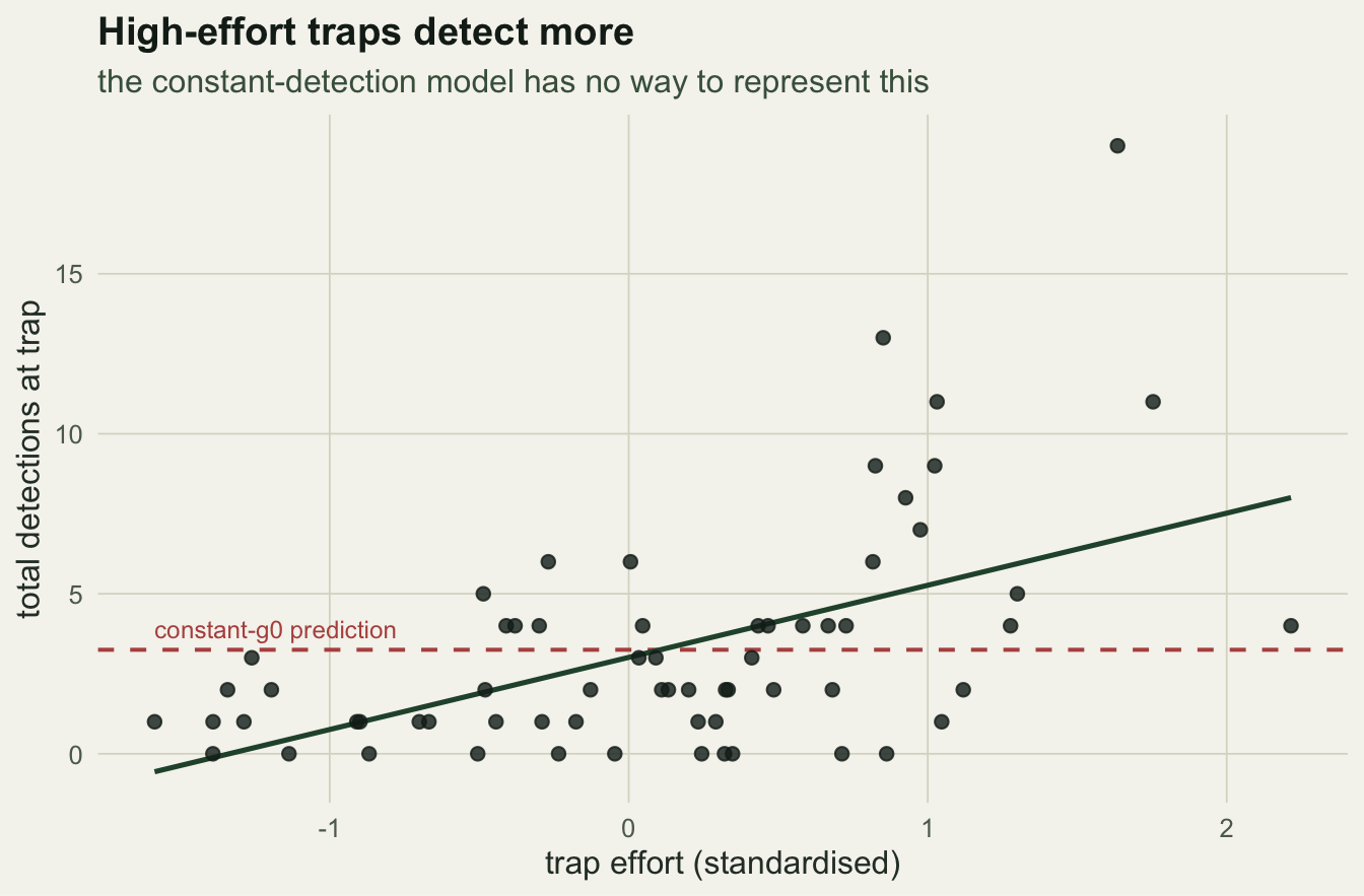
Each trap `j` carries its own baseline `g0j`; high-effort traps detect more. Everything else (the activity-centre integral, the Poisson point process for density) is unchanged from the basics post.
```{r}
#| label: setup
#| code-fold: true
#| code-summary: "Setup: packages, colours and plot theme"
#| results: hide
#| message: false
#| warning: false
library(ggplot2); library(tidyr)
paper <- "#f5f4ee"; ink <- "#16241d"; body <- "#2c3a31"; forest <- "#275139"
labelc <- "#46604a"; sage <- "#93a87f"; linec <- "#dad9ca"; faint <- "#5d6b61"
gold <- "#c9b458"; rust <- "#b5534e"
theme_te <- function(base_size = 12) {
  theme_minimal(base_size = base_size) +
    theme(
      plot.background = element_rect(fill = paper, colour = NA),
      panel.background = element_rect(fill = paper, colour = NA),
      panel.grid.minor = element_blank(),
      panel.grid.major = element_line(colour = linec, linewidth = 0.3),
      axis.title = element_text(colour = body), axis.text = element_text(colour = faint),
      plot.title = element_text(colour = ink, face = "bold"),
      plot.subtitle = element_text(colour = labelc),
      legend.title = element_text(colour = body), legend.text = element_text(colour = body),
      strip.text = element_text(colour = ink, face = "bold")
    )
}
```
```{r}
#| label: sci-tex-helper
#| include: false
sci_tex <- function(x, digits = 2) {
s <- formatC(x, format = "e", digits = digits)
paste0("$", sub("e.*", "", s), " \\times 10^{", as.integer(sub(".*e", "", s)), "}$")
}
```
```{r}
#| label: simulate
set.seed(4130)
tr    <- seq(1, 8, by = 1)
traps <- as.matrix(expand.grid(x = tr, y = tr)); J <- nrow(traps)
K     <- 6
a0_true <- qlogis(0.18); a1_true <- 1.1; sig_true <- 0.75
buffer  <- 3
xl <- range(traps[, 1]) + c(-buffer, buffer); yl <- range(traps[, 2]) + c(-buffer, buffer)
A  <- diff(xl) * diff(yl); N_true <- 90; D_true <- N_true / A

effort <- rnorm(J)                                   # standardised effort per trap
g0_j   <- plogis(a0_true + a1_true * effort)

sx <- runif(N_true, xl[1], xl[2]); sy <- runif(N_true, yl[1], yl[2])
d2 <- outer(sx, traps[, 1], "-")^2 + outer(sy, traps[, 2], "-")^2
P  <- sweep(exp(-d2 / (2 * sig_true^2)), 2, g0_j, "*")
Yf <- matrix(rbinom(N_true * J, K, P), N_true, J)
cc <- rowSums(Yf) > 0; Y <- Yf[cc, , drop = FALSE]; n <- nrow(Y)
trap_tot <- colSums(Y)
```
The study catches `r n` animals with `r sum(Y)` detections and `r sum(rowSums(Y > 0) >= 2)` spatial recaptures.
## Two detection models
We fit two versions of the same integrated likelihood: a null model with a single constant `g0`, and a full model where `g0` depends on effort.
```{r}
#| label: fit
gx <- seq(xl[1], xl[2], length.out = 35); gy <- seq(yl[1], yl[2], length.out = 35)
G  <- as.matrix(expand.grid(x = gx, y = gy))
d2G <- outer(G[, 1], traps[, 1], "-")^2 + outer(G[, 2], traps[, 2], "-")^2
Cc  <- rowSums(lchoose(K, Y))

nll_null <- function(th) {                           # logD, qlogis g0, log sigma
  Dd <- exp(th[1]); g0 <- plogis(th[2]); sg <- exp(th[3])
  Pg <- g0 * exp(-d2G / (2 * sg^2))
  pb <- mean(1 - exp(rowSums(K * log1p(-Pg)))); if (pb <= 0) return(1e10)
  LM <- Y %*% t(log(Pg)) + (K - Y) %*% t(log1p(-Pg)) + Cc
  m  <- apply(LM, 1, max); lf <- m + log(rowMeans(exp(LM - m)))
  -(dpois(n, Dd * A * pb, log = TRUE) + sum(lf) - n * log(pb))
}
nll_full <- function(th) {                           # logD, a0, a1, log sigma
  Dd <- exp(th[1]); gj <- plogis(th[2] + th[3] * effort); sg <- exp(th[4])
  Pg <- sweep(exp(-d2G / (2 * sg^2)), 2, gj, "*")
  pb <- mean(1 - exp(rowSums(K * log1p(-Pg)))); if (pb <= 0) return(1e10)
  LM <- Y %*% t(log(Pg)) + (K - Y) %*% t(log1p(-Pg)) + Cc
  m  <- apply(LM, 1, max); lf <- m + log(rowMeans(exp(LM - m)))
  -(dpois(n, Dd * A * pb, log = TRUE) + sum(lf) - n * log(pb))
}
f0 <- optim(c(log(n/(A*0.4)), qlogis(0.18), log(0.8)), nll_null,
            method = "BFGS", hessian = TRUE, control = list(maxit = 500, reltol = 1e-10))
f1 <- optim(c(log(n/(A*0.4)), a0_true, 1.0, log(0.8)), nll_full,
            method = "BFGS", hessian = TRUE, control = list(maxit = 500, reltol = 1e-10))
stopifnot(f1$convergence == 0)   # check before inverting the Hessian
a1h <- f1$par[3]; se1 <- sqrt(diag(solve(f1$hessian)))
aic0 <- 2*f0$value + 2*length(f0$par); aic1 <- 2*f1$value + 2*length(f1$par)
lrt  <- 2*(f0$value - f1$value); lrt_p <- pchisq(lrt, 1, lower.tail = FALSE)
D0 <- exp(f0$par[1]); g0_0 <- plogis(f0$par[2]); sig0 <- exp(f0$par[3])
D1 <- exp(f1$par[1]); sig1 <- exp(f1$par[4])
```
The full model recovers the effort effect (`a1` estimated at `r round(a1h, 3)` with standard error `r round(se1[3], 3)`, against the true `r a1_true`) and is strongly preferred: the likelihood-ratio statistic is `r round(lrt, 1)` on one degree of freedom (p below `r sci_tex(lrt_p, 1)`), and the effort model has an AIC lower by `r round(aic0 - aic1, 1)`. Both models return almost the same density (`r sprintf("%.3f", D0)` null, `r sprintf("%.3f", D1)` full), so on density alone you might never notice the null model is wrong. That is exactly why a fit check matters.
## Does the detection model fit?
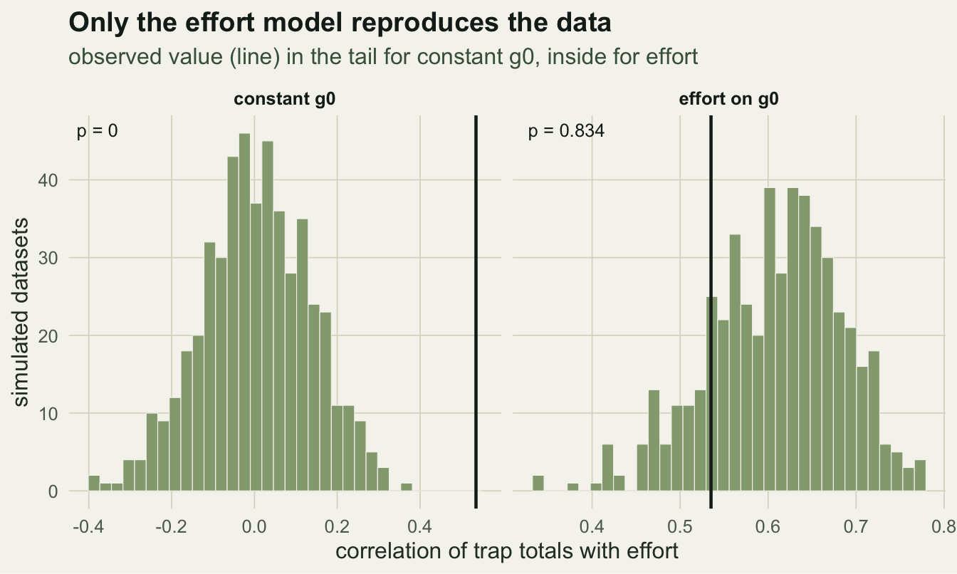
A parametric-bootstrap goodness-of-fit test asks whether a summary of the data is reproducible by the fitted model. The natural summary for a detection covariate is the correlation between each trap's total detections and its effort. Simulate many datasets from a fitted model, compute the statistic each time, and see where the observed value falls.
```{r}
#| label: gof
Tstat <- function(Ymat) cor(colSums(Ymat), effort)
T_obs <- Tstat(Y)

sim_data <- function(D, sg, gj) {                    # gj is the trap-level g0 vector
  Ns <- rpois(1, D * A)
  xs <- runif(Ns, xl[1], xl[2]); ys <- runif(Ns, yl[1], yl[2])
  d2s <- outer(xs, traps[, 1], "-")^2 + outer(ys, traps[, 2], "-")^2
  Yz  <- matrix(rbinom(Ns * J, K, sweep(exp(-d2s / (2 * sg^2)), 2, gj, "*")), Ns, J)
  Yz[rowSums(Yz) > 0, , drop = FALSE]
}
set.seed(77)
B  <- 500
T0 <- replicate(B, Tstat(sim_data(D0, sig0, rep(g0_0, J))))               # null model
T1 <- replicate(B, Tstat(sim_data(D1, sig1, plogis(f1$par[2] + a1h * effort))))  # full model
p0 <- mean(T0 >= T_obs); p1 <- mean(T1 >= T_obs)
```
The observed correlation between trap totals and effort is `r round(T_obs, 3)`. Under the constant-detection model it should be near zero, and it is: the null model's simulated correlations centre on `r round(median(T0), 3)` and the observed value falls far in the upper tail (p < `r sprintf("%.3f", 1/B)`), a clear failure. Under the effort model the simulated correlations centre on `r round(median(T1), 3)` and the observed value sits comfortably inside (p = `r round(p1, 3)`). Same density from both models, but only one reproduces how detections are distributed across traps.
```{r}
#| label: fig-effort
#| fig-cap: "Trap-level total detections against trap effort. Each point is a trap. The rising trend (line) is what the effort model captures; the constant-detection model predicts no dependence on effort (dashed horizontal line at the mean), which the data plainly contradict."
#| fig-alt: "A scatter of trap total detections against standardised effort with a clear upward linear trend line, and a dashed horizontal line at the overall mean showing the flat prediction of the constant-detection model."
#| fig-width: 7
#| fig-height: 4.6
td <- data.frame(effort = effort, total = trap_tot)
p1p <- ggplot(td, aes(effort, total)) +
  geom_hline(yintercept = mean(trap_tot), colour = rust, linetype = "dashed", linewidth = 0.7) +
  geom_smooth(method = "lm", formula = y ~ x, se = FALSE, colour = forest, linewidth = 0.9) +
  geom_point(colour = ink, size = 2, alpha = 0.8) +
  annotate("text", x = min(effort), y = mean(trap_tot), label = "constant-g0 prediction",
           vjust = -0.7, hjust = 0, colour = rust, size = 3.2) +
  labs(x = "trap effort (standardised)", y = "total detections at trap",
       title = "High-effort traps detect more",
       subtitle = "the constant-detection model has no way to represent this") +
  theme_te()
p1p
```
```{r}
#| label: fig-gof
#| fig-cap: "Parametric-bootstrap goodness-of-fit. Simulated trap-effort correlations under each fitted model, with the observed value (solid line). The constant-detection model cannot generate the observed association and places it far in the tail; the effort model contains it."
#| fig-alt: "Two histograms of simulated correlation statistics: the constant-g0 panel centres near zero with the observed value marked far to the right in the tail, and the effort panel centres near the observed value which sits inside the bulk."
#| fig-width: 7
#| fig-height: 4.2
gof <- rbind(data.frame(stat = T0, model = "constant g0"),
             data.frame(stat = T1, model = "effort on g0"))
labs_df <- data.frame(model = c("constant g0", "effort on g0"),
                      lab = c(paste0("p = ", round(p0, 3)), paste0("p = ", round(p1, 3))))
p2p <- ggplot(gof, aes(stat)) +
  geom_histogram(bins = 34, fill = sage, colour = paper, linewidth = 0.2) +
  geom_vline(xintercept = T_obs, colour = ink, linewidth = 0.8) +
  geom_text(data = labs_df, aes(x = -Inf, y = Inf, label = lab),
            hjust = -0.2, vjust = 1.6, colour = ink, size = 3.4, inherit.aes = FALSE) +
  facet_wrap(~ model, scales = "free_x") +
  labs(x = "correlation of trap totals with effort", y = "simulated datasets",
       title = "Only the effort model reproduces the data",
       subtitle = "observed value (line) in the tail for constant g0, inside for effort") +
  theme_te()
p2p
```
```{r}
#| label: thumb
#| include: false
ggsave("thumbnail.png", p2p + labs(title = NULL, subtitle = NULL),
width = 7.5, height = 5.4, dpi = 100, bg = paper)
```
## Takeaways
Detection covariates belong in the SCR detection function whenever effort or conditions vary across traps, and adding one is a small change: the baseline `g0` becomes a logit-linear function of the covariate inside the same likelihood. The subtler point is that density can look fine while the detection model is wrong, so a fit check is not optional. A parametric bootstrap makes it concrete: pick a statistic the covariate should affect (here the trap-total to effort correlation), simulate from the fitted model, and see whether the observed value is reproducible. The constant-detection model fails that test decisively while giving a plausible density; the effort model passes. This closes the spatial capture-recapture series: estimate density, do it the Bayesian way, design the array, and check the detection model that everything rests on.
## References
Borchers DL, Efford MG 2008 Biometrics 64(2):377-385 (10.1111/j.1541-0420.2007.00927.x)
Efford MG, Borchers DL, Byrom AE 2009 In: Modeling Demographic Processes in Marked Populations, Springer (10.1007/978-0-387-78151-8_11)
Royle JA, Karanth KU, Gopalaswamy AM, Kumar NS 2009 Ecology 90(11):3233-3244 (10.1890/08-1481.1)
Efford M 2004 Oikos 106(3):598-610 (10.1111/j.0030-1299.2004.13043.x)
Royle JA, Chandler RB, Sollmann R, Gardner B 2014 Spatial Capture-Recapture. Academic Press (ISBN 978-0-12-405939-9)
## Related tutorials
- [Spatial capture-recapture from scratch](../spatial-capture-recapture-basics/)
- [SCR sampling design and precision](../scr-sampling-design/)
- [Bayesian spatial capture-recapture](../bayesian-spatial-capture-recapture/)
- [Trap-specific responses in spatial capture-recapture](../trap-specific-responses-in-scr/)