library(survival)
library(ggplot2)
library(patchwork)

te_paper  <- "#f5f4ee"
te_ink    <- "#16241d"
te_body   <- "#2c3a31"
te_forest <- "#275139"
te_rust   <- "#b5534e"
te_gold   <- "#c9b458"
te_line   <- "#dad9ca"

theme_datasheet <- function() {
  theme_minimal(base_size = 12) +
    theme(plot.background  = element_rect(fill = te_paper, colour = NA),
          panel.background = element_rect(fill = te_paper, colour = NA),
          panel.grid.major = element_line(colour = te_line, linewidth = 0.3),
          panel.grid.minor = element_blank(),
          text             = element_text(colour = te_body),
          plot.title       = element_text(colour = te_ink, face = "bold"),
          plot.subtitle    = element_text(colour = te_body),
          axis.text        = element_text(colour = te_body))
}Missing GPS fixes in step selection
R
movement ecology
habitat selection
telemetry
missing data
simulation
ecology tutorial
GPS fixes fail under cover. Dropping irregular steps biases step selection, bridging the gaps trades one bias for another, and weights cost precision. In R.
A GPS collar on a forest deer is set to try for a position every hour. In open ground almost every attempt returns a fix; under dense cover a good share of them come back empty. The track that reaches the analyst is a regular schedule with holes in it, and an integrated step selection analysis wants something else: a sequence of steps of equal duration, each compared with the steps the animal could have taken from the same start. The usual preparation resamples the track to the schedule and keeps only the steps between two consecutive successful fixes, so every step that touches a gap is dropped. The alternative is to bridge the gap: keep the step from the last fix before it to the first fix after it, and tell the model that this step lasted two or three intervals instead of one.
Hofmann, Cozzi and Fieberg (2024) reassessed the dropping rule and compared ways of keeping the irregular steps, including a model that fits a separate movement kernel for each step duration and lets the movement terms interact with duration, bridging gaps up to a maximum duration they call forgiveness. Their fixes were removed at random, and for the scenarios they simulated the habitat-selection estimates were insensitive to the inclusion of irregular data. In their discussion they add that fix loss is often not random, citing studies that tie it to topography, canopy cover, time of day, animal behaviour and collar orientation. Loss that follows the habitat being selected is the subject here. Nothing in this post is a new estimator; it runs the dropping rule, the inverse-probability weights and the duration-aware bridge side by side on the same tracks, under random loss and under loss that follows the habitat being selected, against the fit to the complete track.
The dropping half of the result is not new on this site. GPS fix loss and the collars you drop shows, for a resource selection function, that fixes lost under canopy thin the used points by the fix probability and shift the canopy coefficient by roughly the slope of the log fix probability, and that weighting each acquired fix by one over its fix probability removes the shift, with the true fix model and also with one estimated from stationary test collars, provided the test sites span the canopy range. That mechanism carries over to steps unchanged, and it is credited to that post and to Frair and colleagues (2004) wherever it appears below. What the resource selection function has no counterpart for is the bridge. The conditional logistic machinery is the one built in step selection functions for animal movement, with the step-length terms of integrated step selection analysis and ten available steps per used step, a choice discussed in availability sampling for step selection; every track in those posts is complete and regular. A gappy track can also be regularised with a continuous-time smoother, as in regularising irregular animal tracks, but that post never feeds its reconstruction to a step selection model, and imputing the missing positions is not one of the arms run here.
A walker, a cover layer and a collar that fails
The landscape is one smooth covariate, called cover here, built from three sine waves and bounded by -2.5 and 2.5, the sum of their amplitudes. At every time step the animal draws 30 candidate moves from a movement kernel, a gamma step length with shape 2 and scale 1.5 (mean 3 units) and a uniform direction, and takes one of them with probability proportional to exp(beta * cover) at its end, with beta equal to 1. The choice is made with the Gumbel-max trick, which draws from exactly those probabilities and vectorises over tracks. The animal has no directional persistence, so turning angles carry nothing and the available steps below use uniform directions.
The collar tries for a fix at every time step and fails with a probability that depends on the cover at the animal’s true position, through a logistic model. Three loss models are run. Under random loss the failure probability is 0.3 or 0.6 everywhere. Under steep cover-dependent loss it is 0.3 at a cover of zero with a logistic slope of 1.5, a deliberately severe setting. Under moderate cover-dependent loss it is fixed by two anchor points chosen before any run: 0.05 at a cover of -2 and 0.5 at a cover of 2. The steep model is also run on an animal that ignores cover (beta of 0), as a placebo. Each track has 1500 steps, and every setting is run on 120 tracks, which puts a Monte Carlo standard error on every compared mean.
hab_curved <- function(x, y) sin(x / 7) + cos(y / 9) + 0.5 * sin((x + y) / 5)
beta_sel    <- 1
n_cand      <- 30
step_shape  <- 2
step_scale  <- 1.5
n_step      <- 1500
n_avail     <- 10
n_trk       <- 120
caps        <- c(2, 3, 5, Inf)
lump_dt     <- 5
min_group   <- 30

steep_a0    <- qlogis(0.3)
steep_slope <- 1.5
mod_slope   <- (qlogis(0.5) - qlogis(0.05)) / 4
mod_a0      <- qlogis(0.5) - 2 * mod_slope
p_loss <- function(h, a0, slope) plogis(a0 + slope * h)
wave_len <- 2 * pi * c(7, 9, 5 / sqrt(2))
The three waves have wavelengths of 22, 44 and 57 distance units, against a mean step length of 3, so cover changes smoothly over one step and appreciably over a few.
sim_tracks <- function(n_tr, beta, hfun = hab_curved) {
  px <- matrix(0, n_tr, n_step + 1)
  py <- px
  n_draw <- n_tr * n_cand
  for (tt in seq_len(n_step)) {
    len <- matrix(rgamma(n_draw, step_shape, scale = step_scale), n_tr)
    ang <- matrix(runif(n_draw, 0, 2 * pi), n_tr)
    cand_x <- px[, tt] + len * cos(ang)
    cand_y <- py[, tt] + len * sin(ang)
    score <- beta * hfun(cand_x, cand_y) - log(-log(matrix(runif(n_draw), n_tr)))
    pick <- cbind(seq_len(n_tr), max.col(score, ties.method = "first"))
    px[, tt + 1] <- cand_x[pick]
    py[, tt + 1] <- cand_y[pick]
  }
  list(x = px, y = py)
}
The model fitted to every version of a track is the step selection function of Fortin and colleagues (2005) with the movement terms of integrated step selection analysis (Avgar and colleagues 2016): cover at the end of the step, step length and log step length, in a conditional logistic likelihood with one stratum per used step and ten available steps drawn from a gamma fitted by moments to the observed step lengths. It is fitted by Newton-Raphson with optional stratum weights, because 120 tracks times several arms times several settings is too many calls to clogit() for a page that knits in a few minutes. The chunk checks it on one gappy track against clogit() for the duration-aware model and against a weighted coxph() fit for the weighted one.
make_strata <- function(x, y, keep, mode, cap = Inf, hfun = hab_curved) {
  idx <- which(keep)
  dur <- diff(idx)
  from <- idx[-length(idx)]
  to <- idx[-1]
  ok <- if (mode == "drop") dur == 1 else dur <= cap
  from <- from[ok]
  to <- to[ok]
  dur <- dur[ok]
  len <- sqrt((x[to] - x[from])^2 + (y[to] - y[from])^2)
  grp <- if (mode == "aware") pmin(dur, lump_dt) else rep(1, length(dur))
  if (mode == "aware") {
    for (g in sort(unique(grp), decreasing = TRUE)) {
      if (g > 1 && sum(grp == g) < min_group) grp[grp == g] <- g - 1
    }
  }
  n_s <- length(len)
  shp <- scl <- numeric(n_s)
  for (g in unique(grp)) {
    v <- len[grp == g]
    shp[grp == g] <- mean(v)^2 / var(v)
    scl[grp == g] <- var(v) / mean(v)
  }
  av_len <- matrix(rgamma(n_s * n_avail, rep(shp, n_avail), scale = rep(scl, n_avail)), n_s)
  av_ang <- matrix(runif(n_s * n_avail, 0, 2 * pi), n_s)
  end_x <- cbind(x[to], x[from] + av_len * cos(av_ang))
  end_y <- cbind(y[to], y[from] + av_len * sin(av_ang))
  sl_mat <- cbind(len, av_len)
  list(h = hfun(end_x, end_y), sl = sl_mat, lsl = log(sl_mat), grp = grp, dur = dur)
}

design_of <- function(st, aware) {
  out <- list(h = st$h)
  lev <- if (aware) sort(unique(st$grp)) else 1
  for (g in lev) {
    on <- if (aware) st$grp == g else rep(TRUE, length(st$grp))
    out[[paste0("sl_", g)]] <- st$sl * on
    out[[paste0("lsl_", g)]] <- st$lsl * on
  }
  out
}

subset_strata <- function(st, ok) {
  list(h = st$h[ok, , drop = FALSE], sl = st$sl[ok, , drop = FALSE],
       lsl = st$lsl[ok, , drop = FALSE], grp = st$grp[ok], dur = st$dur[ok])
}
fit_clogit <- function(xl, wt = NULL, iter = 50) {
n_par <- length(xl)
n_s <- nrow(xl[[1]])
n_c <- ncol(xl[[1]])
if (is.null(wt)) wt <- rep(1, n_s)
row_max <- function(m) m[cbind(seq_len(n_s), max.col(m, "first"))]
lin_pred <- function(b) {
eta <- xl[[1]] * b[1]
if (n_par > 1) for (k in 2:n_par) eta <- eta + xl[[k]] * b[k]
eta
}
loglik <- function(b) {
eta <- lin_pred(b)
mx <- row_max(eta)
sum(wt * (eta[, 1] - mx - log(.rowSums(exp(eta - mx), n_s, n_c))))
}
b <- rep(0, n_par)
ll <- loglik(b)
for (it in seq_len(iter)) {
eta <- lin_pred(b)
pr <- exp(eta - row_max(eta))
pr <- pr / .rowSums(pr, n_s, n_c)
x_bar <- vapply(xl, function(m) .rowSums(pr * m, n_s, n_c), numeric(n_s))
x_use <- vapply(xl, function(m) m[, 1], numeric(n_s))
grad <- colSums(wt * (x_use - x_bar))
hess <- matrix(0, n_par, n_par)
for (k in seq_len(n_par)) {
pk <- pr * xl[[k]]
for (l in k:n_par) {
hess[k, l] <- hess[l, k] <-
sum(wt * (.rowSums(pk * xl[[l]], n_s, n_c) - x_bar[, k] * x_bar[, l]))
}
}
step <- solve(hess, grad)
fac <- 1
repeat {
b_new <- b + fac * step
ll_new <- loglik(b_new)
if (ll_new >= ll - 1e-9 || fac < 1e-4) break
fac <- fac / 2
}
done <- abs(ll_new - ll) < 1e-10
b <- b_new
ll <- ll_new
if (done) break
}
setNames(b, names(xl))
}
long_frame <- function(st) {
n_s <- nrow(st$h)
n_c <- ncol(st$h)
data.frame(stratum = rep(seq_len(n_s), n_c), case = rep(c(1, rep(0, n_c - 1)), each = n_s),
h = c(st$h), sl = c(st$sl), lsl = c(st$lsl), dgrp = factor(rep(st$grp, n_c)))
}
set.seed(3701)
chk_trk <- sim_tracks(1, beta_sel)
chk_x <- chk_trk$x[1, ]
chk_y <- chk_trk$y[1, ]
chk_keep <- runif(n_step + 1) > 0.6
chk_keep[1] <- TRUE
chk_aw <- make_strata(chk_x, chk_y, chk_keep, "aware")
own_aw <- fit_clogit(design_of(chk_aw, TRUE))[["h"]]
pkg_aw <- coef(clogit(case ~ h + sl:dgrp + lsl:dgrp + strata(stratum),
data = long_frame(chk_aw)))[["h"]]
chk_dr <- make_strata(chk_x, chk_y, chk_keep, "drop")
chk_w <- runif(nrow(chk_dr$h), 1, 4)
chk_frame <- long_frame(chk_dr)
chk_frame$w <- chk_w[chk_frame$stratum]
own_w <- fit_clogit(design_of(chk_dr, FALSE), chk_w)[["h"]]
pkg_w <- coef(coxph(Surv(rep(1, nrow(chk_frame)), case) ~ h + sl + lsl + strata(stratum),
data = chk_frame, weights = w, method = "breslow"))[["h"]]
fit_gap <- max(abs(own_aw - pkg_aw), abs(own_w - pkg_w))
stopifnot(fit_gap < 1e-6)On a track with 894 of 1501 fixes missing, the hand-written fit gives a cover coefficient of 0.956693 for the duration-aware model and clogit() gives 0.956693; with random stratum weights the two weighted fits give 0.563150 and 0.563150. The largest difference is \(3.71 \times 10^{-10}\).
Four ways to handle a gap
Every track is analysed five ways, and all five are compared with the first.
The complete track, every position present and every step one interval long, is the reference no field study has. Its coefficient comes out a little below 1, because an animal choosing among 30 candidates only approximates the continuous model and the fitted gamma only approximates the observed step lengths. Everything below is therefore measured as a paired difference from the complete-track fit of the same track.
Dropping keeps only the steps between two consecutive successful fixes, the regular bursts of Hofmann and colleagues.
Dropping with weights keeps the same steps and gives each stratum the weight one over the probability that the fix at the end of its step was obtained, computed from the true fix model at the true position. This is the Horvitz-Thompson weight (Horvitz and Thompson 1952) of the fix-loss post, placed on the same unit, the acquired fix: a stratum holds exactly one used fix, and weighting the stratum is weighting that fix’s contribution to the likelihood. The fix at the start of the step also had to succeed, but the start is what the stratum conditions on, so its probability changes how much a stratum counts and not what it estimates; that claim is tested below. In a real study the fix model is not known and is estimated from stationary test collars, as the fix-loss post does, and its error adds to what is shown here.
The one-kernel bridge turns every pair of consecutive successful fixes into a step, whatever its duration, and fits one gamma and one pair of step-length terms to all of them.
The duration-aware bridge follows Hofmann and colleagues: a separate gamma for each step duration, the available steps of a bridged step drawn from the gamma of its own duration, and the step-length and log step-length terms interacted with duration, so that only the cover coefficient is shared. Durations of five intervals or more share one kernel, and a duration class with fewer than 30 steps in a track is merged into the next shorter one. It is run with a forgiveness of 2, 3 and 5 intervals, and with every gap bridged.
one_track <- function(x, y, a0, slope, extra = FALSE) {
  n1 <- length(x)
  pl <- p_loss(hab_curved(x, y), a0, slope)
  keep <- runif(n1) > pl
  keep[1] <- TRUE
  st_full <- make_strata(x, y, rep(TRUE, n1), "drop")
  st_drop <- make_strata(x, y, keep, "drop")
  w_end <- 1 / (1 - p_loss(st_drop$h[, 1], a0, slope))
  st_all <- make_strata(x, y, keep, "aware")
  cap_fit <- vapply(caps, function(cp) {
    st <- if (is.infinite(cp)) st_all else make_strata(x, y, keep, "aware", cap = cp)
    fit_clogit(design_of(st, TRUE))[["h"]]
  }, 0)
  out <- c(full = fit_clogit(design_of(st_full, FALSE))[["h"]],
           drop = fit_clogit(design_of(st_drop, FALSE))[["h"]],
           ipw = fit_clogit(design_of(st_drop, FALSE), w_end)[["h"]],
           one = fit_clogit(design_of(make_strata(x, y, keep, "one"), FALSE))[["h"]],
           cap_2 = cap_fit[1], cap_3 = cap_fit[2], cap_5 = cap_fit[3], cap_all = cap_fit[4],
           got = mean(keep), regular = nrow(st_drop$h) / (n1 - 1),
           share_3 = mean(st_all$dur >= 3))
  if (extra) {
    kept <- which(keep)
    reg <- which(diff(kept) == 1)
    w_both <- w_end / (1 - p_loss(hab_curved(x[kept[reg]], y[kept[reg]]), a0, slope))
    avail_h <- st_drop$h[, -1]
    avail_lq <- log(1 - p_loss(avail_h, a0, slope))
    dev_h <- avail_h - rowMeans(avail_h)
    dev_lq <- avail_lq - rowMeans(avail_lq)
    dur_fit <- function(ok) fit_clogit(design_of(subset_strata(st_all, ok), TRUE))[["h"]]
    out <- c(out,
             ipw_both = fit_clogit(design_of(st_drop, FALSE), w_both)[["h"]],
             logq_slope = sum(dev_h * dev_lq) / sum(dev_h^2),
             dur_1 = dur_fit(st_all$dur == 1), dur_2 = dur_fit(st_all$dur == 2),
             dur_3 = dur_fit(st_all$dur >= 3))
  }
  out
}

run_setting <- function(beta, a0, slope, extra = FALSE, keep_paths = FALSE) {
  trk <- sim_tracks(n_trk, beta)
  res <- t(vapply(seq_len(n_trk), function(i)
    one_track(trk$x[i, ], trk$y[i, ], a0, slope, extra), numeric(if (extra) 16 else 11)))
  list(est = as.data.frame(res), paths = if (keep_paths) trk else NULL)
}

set.seed(4801)
sc_r30 <- run_setting(beta_sel, qlogis(0.3), 0, keep_paths = TRUE)
set.seed(4802)
sc_r60 <- run_setting(beta_sel, qlogis(0.6), 0, extra = TRUE)
set.seed(4803)
sc_st1 <- run_setting(beta_sel, steep_a0, steep_slope, extra = TRUE)
set.seed(4804)
sc_st0 <- run_setting(0, steep_a0, steep_slope, extra = TRUE)
set.seed(4805)
sc_md1 <- run_setting(beta_sel, mod_a0, mod_slope, extra = TRUE)

settings <- list(r30 = sc_r30, r60 = sc_r60, st1 = sc_st1, st0 = sc_st0, md1 = sc_md1)
set_lab <- c(r30 = "random loss 0.3", r60 = "random loss 0.6", st1 = "steep, cover selected",
             st0 = "steep, cover ignored", md1 = "moderate, cover selected")
arm_names <- c("full", "drop", "ipw", "one", "cap_2", "cap_3", "cap_5", "cap_all")
tab <- do.call(rbind, lapply(names(settings), function(k) {
  e <- settings[[k]]$est
  do.call(rbind, lapply(arm_names, function(a) data.frame(
    key = k, arm = a, mean = mean(e[[a]]), sd = sd(e[[a]]),
    diff = mean(e[[a]] - e$full), diff_se = sd(e[[a]] - e$full) / sqrt(n_trk))))
}))
val <- function(k, a, col = "diff") tab[tab$key == k & tab$arm == a, col]
ext <- function(k, v) mean(settings[[k]]$est[[v]])
ext_sd <- function(k, v) sd(settings[[k]]$est[[v]])
print(tab[tab$arm %in% c("full", "drop", "ipw", "one", "cap_all"), ], digits = 3, row.names = FALSE)
key arm mean sd diff diff_se
r30 full 0.96543 0.0848 0.000000 0.00000
r30 drop 0.96600 0.1379 0.000561 0.00942
r30 ipw 0.96600 0.1379 0.000561 0.00942
r30 one 0.99270 0.0957 0.027262 0.00428
r30 cap_all 1.00693 0.0867 0.041496 0.00393
r60 full 0.97294 0.0888 0.000000 0.00000
r60 drop 1.00343 0.2115 0.030486 0.01774
r60 ipw 1.00343 0.2115 0.030486 0.01774
r60 one 1.06453 0.1014 0.091583 0.00557
r60 cap_all 1.11043 0.1076 0.137487 0.00563
st1 full 0.95365 0.0873 0.000000 0.00000
st1 drop 0.24025 0.2797 -0.713399 0.02484
st1 ipw 0.96264 0.3792 0.008990 0.03380
st1 one 0.56862 0.1096 -0.385037 0.00674
st1 cap_all 0.80634 0.1147 -0.147309 0.00638
st0 full 0.00085 0.0656 0.000000 0.00000
st0 drop -0.32135 0.0868 -0.322200 0.00709
st0 ipw -0.01118 0.1192 -0.012029 0.00917
st0 one -0.21395 0.0646 -0.214802 0.00403
st0 cap_all -0.09462 0.0653 -0.095471 0.00341
md1 full 0.97074 0.0865 0.000000 0.00000
md1 drop 0.70606 0.1501 -0.264674 0.01050
md1 ipw 0.96710 0.1630 -0.003638 0.01135
md1 one 0.85996 0.0899 -0.110776 0.00447
md1 cap_all 0.97048 0.0978 -0.000263 0.00422The table printed above is the whole experiment in five settings. The figure shows the per-track differences from the complete track for the four arms that handle a gap, with every gap bridged in the duration-aware arm.
arm_show <- c(drop = "drop", ipw = "drop +\nweights", one = "bridge,\none kernel",
              cap_all = "bridge,\nby duration")
arm_long <- do.call(rbind, lapply(names(settings), function(k) {
  e <- settings[[k]]$est
  do.call(rbind, lapply(names(arm_show), function(a)
    data.frame(setting = set_lab[[k]], arm = arm_show[[a]], d = e[[a]] - e$full)))
}))
arm_long$arm <- factor(arm_long$arm, levels = arm_show)
arm_long$setting <- factor(arm_long$setting, levels = set_lab[c("r30", "r60", "md1", "st1", "st0")])
set.seed(73)
ggplot(arm_long, aes(arm, d)) +
  geom_hline(yintercept = 0, colour = te_ink, linewidth = 0.5) +
  geom_jitter(width = 0.17, height = 0, size = 0.9, alpha = 0.4, colour = te_forest) +
  stat_summary(fun = mean, geom = "point", shape = 23, size = 3.2,
               fill = te_rust, colour = te_paper) +
  facet_wrap(~ setting, ncol = 3) +
  labs(x = NULL, y = "difference from the complete track",
       title = "Only the weights are centred in all five settings",
       subtitle = "points: tracks; diamonds: means over 120 tracks") +
  theme_datasheet() +
  theme(strip.text = element_text(colour = te_ink, face = "bold"))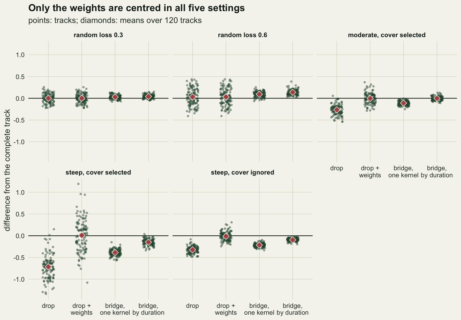
Random loss: dropping costs precision, bridging leans high
When fixes fail at random, which steps survive has nothing to do with where they end, and the regular steps are a random subset of the track. A step survives when both of its fixes do, so with a loss probability q (a fix probability 1 - q) a share (1 - q)^2 of the steps is left in expectation, and the standard deviation of the coefficient grows by about 1 / (1 - q). That is arithmetic, derived rather than found; the chunk sets it against the measured spread.
reg_30 <- ext("r30", "regular")
reg_60 <- ext("r60", "regular")
sd_ratio_30 <- val("r30", "drop", "sd") / val("r30", "full", "sd")
sd_ratio_60 <- val("r60", "drop", "sd") / val("r60", "full", "sd")
set.seed(4807)
boot_i <- replicate(2000, sample.int(n_trk, replace = TRUE))
log_ratio_se <- function(k) sd(apply(boot_i, 2, function(i)
  log(sd(settings[[k]]$est$drop[i]) / sd(settings[[k]]$est$full[i]))))
ratio_z_30 <- log(sd_ratio_30 * 0.7) / log_ratio_se("r30")
ratio_z_60 <- log(sd_ratio_60 * 0.4) / log_ratio_se("r60")
cap_tab <- tab[tab$arm %in% c("drop", "cap_2", "cap_3", "cap_5", "cap_all"), ]
pct_30 <- 100 * val("r30", "cap_all") / val("r30", "full", "mean")
pct_60 <- 100 * val("r60", "cap_all") / val("r60", "full", "mean")
print(cap_tab, digits = 3, row.names = FALSE)
key arm mean sd diff diff_se
r30 drop 0.9660 0.1379 0.000561 0.00942
r30 cap_2 0.9855 0.0984 0.020045 0.00547
r30 cap_3 1.0057 0.0948 0.040224 0.00502
r30 cap_5 1.0084 0.0894 0.042949 0.00384
r30 cap_all 1.0069 0.0867 0.041496 0.00393
r60 drop 1.0034 0.2115 0.030486 0.01774
r60 cap_2 1.0092 0.1611 0.036271 0.01269
r60 cap_3 1.0332 0.1397 0.060237 0.01032
r60 cap_5 1.0725 0.1175 0.099558 0.00770
r60 cap_all 1.1104 0.1076 0.137487 0.00563
st1 drop 0.2403 0.2797 -0.713399 0.02484
st1 cap_2 0.3453 0.1852 -0.608398 0.01586
st1 cap_3 0.4281 0.1506 -0.525587 0.01291
st1 cap_5 0.5274 0.1411 -0.426302 0.01168
st1 cap_all 0.8063 0.1147 -0.147309 0.00638
st0 drop -0.3214 0.0868 -0.322200 0.00709
st0 cap_2 -0.2351 0.0731 -0.235994 0.00567
st0 cap_3 -0.1953 0.0688 -0.196196 0.00531
st0 cap_5 -0.1478 0.0688 -0.148669 0.00450
st0 cap_all -0.0946 0.0653 -0.095471 0.00341
md1 drop 0.7061 0.1501 -0.264674 0.01050
md1 cap_2 0.8097 0.1118 -0.160996 0.00652
md1 cap_3 0.8738 0.1058 -0.096902 0.00548
md1 cap_5 0.9357 0.0938 -0.035064 0.00421
md1 cap_all 0.9705 0.0978 -0.000263 0.00422With a loss probability of 0.3 the regular steps are 0.491 of the track against an expected 0.49, and with 0.6 they are 0.159 against 0.16. The standard deviation of the dropped-step coefficient across tracks is 1.62 and 2.38 times that of the complete track, against 1.43 and 2.50 from the step count. A bootstrap over the 120 tracks, resampling each track’s complete and dropped fits together, puts the log of the measured ratio +2.2 bootstrap standard errors from the step-count value at 0.3 (a positive sign means noisier than the step count predicts) and -0.6 at 0.6: the step count gives the size of the cost, and a gap of that size in one setting on one set of tracks is not a finding either way. The mean difference from the complete track is +0.001 (Monte Carlo standard error 0.009) and +0.030 (0.018), neither further than two standard errors from zero. The weights change nothing under random loss, because every weight is the same; that arm is the dropping arm by construction.
Bridging keeps the steps and pays with a bias. With every gap bridged, the duration-aware model sits +0.041 above the complete track at a loss probability of 0.3 (standard error 0.004), about 4 per cent of the coefficient, and +0.137 at 0.6 (0.006), about 14 per cent. The one-kernel bridge is +0.027 and +0.092. At the lower loss the shift is small, and Hofmann and colleagues, on their own simulated layers, found the habitat estimates insensitive to including the irregular steps; at the higher loss it is not small. The shift also grows with the longest gap allowed: at 0.6 it is +0.036 with a forgiveness of 2 intervals, +0.060 with 3, +0.100 with 5, and +0.137 with every gap bridged.
Why a longer step read as stronger selection here
The bridged steps are not wrong steps. Each is the real displacement over two or more intervals, and its available steps come from the kernel of that duration. Where the upward lean comes from can be seen by removing the gaps from the question: take a complete track, keep every second or third fix, and fit the model to the resulting regular two- or three-interval steps.
On a plane, where cover rises in a straight line with gradient g, the answer can be written down. A one-interval displacement d has density proportional to k(d) exp(beta * g . d), the same everywhere on the plane. The displacement over two intervals is the sum of two independent one-interval displacements, and because exp(beta * g . d1) * exp(beta * g . d2) = exp(beta * g . (d1 + d2)), its density is the two-interval movement kernel tilted by exp(beta * g . D): the same exponential selection with the same beta. A model fitted to two-interval steps with the two-interval kernel as availability should therefore return beta (exactly so in the limit of a continuous choice; with 30 candidates the tilt of one step is only approximately exponential). On a curved layer the argument breaks at the intermediate position, where the attraction of that position relative to the total attraction of the moves available from it depends on where it is, and does not cancel.
grad_seq <- seq(0, 600, by = 0.5)
grad_pts <- expand.grid(x = grad_seq, y = grad_seq)
d_eps <- 1e-4
grad_x <- (hab_curved(grad_pts$x + d_eps, grad_pts$y) -
           hab_curved(grad_pts$x - d_eps, grad_pts$y)) / (2 * d_eps)
grad_y <- (hab_curved(grad_pts$x, grad_pts$y + d_eps) -
           hab_curved(grad_pts$x, grad_pts$y - d_eps)) / (2 * d_eps)
plane_slope <- sqrt(mean(grad_x^2 + grad_y^2))
hab_plane <- function(x, y) plane_slope * x
intervals <- c(1, 2, 3, 5)

thin_fit <- function(x, y, k, hfun) {
  keep <- rep(FALSE, length(x))
  keep[seq(1, length(x), by = k)] <- TRUE
  fit_clogit(design_of(make_strata(x, y, keep, "one", hfun = hfun), FALSE))[["h"]]
}
set.seed(4806)
thin_curved <- t(vapply(seq_len(n_trk), function(i)
  vapply(intervals, function(k)
    thin_fit(sc_r30$paths$x[i, ], sc_r30$paths$y[i, ], k, hab_curved), 0),
  numeric(length(intervals))))
plane_trk <- sim_tracks(n_trk, beta_sel, hfun = hab_plane)
thin_plane <- t(vapply(seq_len(n_trk), function(i)
  vapply(intervals, function(k)
    thin_fit(plane_trk$x[i, ], plane_trk$y[i, ], k, hab_plane), 0),
  numeric(length(intervals))))
thin_tab <- rbind(
  data.frame(surface = "curved cover layer", interval = intervals,
             diff = colMeans(thin_curved - thin_curved[, 1]),
             se = apply(thin_curved - thin_curved[, 1], 2, sd) / sqrt(n_trk)),
  data.frame(surface = "plane, same mean steepness", interval = intervals,
             diff = colMeans(thin_plane - thin_plane[, 1]),
             se = apply(thin_plane - thin_plane[, 1], 2, sd) / sqrt(n_trk)))
print(thin_tab, digits = 3, row.names = FALSE)
surface interval diff se
curved cover layer 1 0.00000 0.00000
curved cover layer 2 0.08016 0.00461
curved cover layer 3 0.13679 0.00521
curved cover layer 5 0.23249 0.00747
plane, same mean steepness 1 0.00000 0.00000
plane, same mean steepness 2 -0.00368 0.00375
plane, same mean steepness 3 -0.00666 0.00491
plane, same mean steepness 5 0.00373 0.00519plane_z <- abs(thin_tab$diff / thin_tab$se)[thin_tab$surface != "curved cover layer" &
thin_tab$interval > 1]
plane_max_z <- max(plane_z)The check runs both. The curved layer is the cover layer used throughout, thinned from the complete tracks of the first random-loss setting. The plane has a gradient equal to the root mean square gradient of the curved layer, 0.162 per unit distance, so the two surfaces are equally steep on average.
ggplot(thin_tab, aes(interval, diff, colour = surface)) +
  geom_hline(yintercept = 0, colour = te_body, linewidth = 0.4) +
  geom_line(linewidth = 0.9) +
  geom_errorbar(aes(ymin = diff - 2 * se, ymax = diff + 2 * se), width = 0.12, linewidth = 0.6) +
  geom_point(size = 2.6) +
  scale_colour_manual(values = c(te_rust, te_forest), name = NULL) +
  scale_x_continuous(breaks = intervals) +
  labs(x = "fix interval of the thinned track (steps)",
       y = "coefficient minus the one-interval fit",
       title = "Coarser steps read as stronger selection on this layer",
       subtitle = "no fixes lost: every k-th fix of the complete track") +
  theme_datasheet() +
  theme(legend.position = "bottom")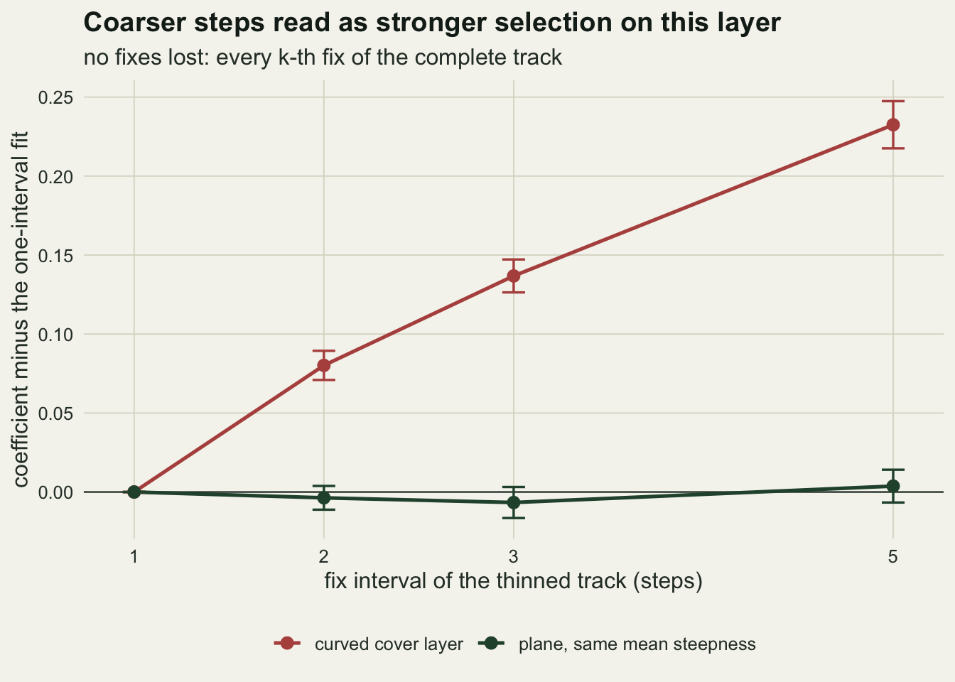
On the curved layer the coefficient rises by 0.080 at 2 intervals, 0.137 at 3 and 0.232 at 5 (standard errors 0.005 to 0.007). On the plane the three differences are -0.004, -0.007 and +0.004, none more than 1.4 standard errors from zero, as the derivation says. So two rounds of selection do not by themselves read as stronger selection. The lean comes from the curvature of the covariate over the distance a multi-interval step covers, and on this layer its sign is upward. A bridge under random loss mixes these coarser steps into a model whose cover coefficient is shared across durations, which is where the shift in the previous section comes from, and why it grows with the longest gap bridged. How large it is in a real landscape depends on how rough the covariate is relative to a bridged displacement, and step lengths and turning angles in R already shows the path metrics themselves changing with the fix interval.
Loss that follows cover: the fix-loss bias, step by step
Now the collar fails more often under cover, and the animal, with beta of 1, spends its time in cover. That is the combination Frair and colleagues (2004) described for resource selection, and the fix-loss post measures.
got_st1 <- ext("st1", "got")
got_st0 <- ext("st0", "got")
got_md1 <- ext("md1", "got")
logq_st1 <- ext("st1", "logq_slope")
logq_st0 <- ext("st0", "logq_slope")
logq_md1 <- ext("md1", "logq_slope")
full_q025 <- quantile(sc_st0$est$full, 0.025)
plc_below <- mean(sc_st0$est$drop < full_q025)
ipw_ratio_st1 <- val("st1", "ipw", "sd") / val("st1", "full", "sd")
ipw_ratio_md1 <- val("md1", "ipw", "sd") / val("md1", "full", "sd")
cover_max <- max(hab_curved(grad_pts$x, grad_pts$y))
w_top_st <- 1 / (1 - p_loss(cover_max, steep_a0, steep_slope))
w_top_md <- 1 / (1 - p_loss(cover_max, mod_a0, mod_slope))
both_st1 <- ext("st1", "ipw_both") - ext("st1", "full")
both_se_st1 <- sd(sc_st1$est$ipw_both - sc_st1$est$full) / sqrt(n_trk)
approx_gap <- max(abs(c(logq_st1 - val("st1", "drop"), logq_st0 - val("st0", "drop"),
                        logq_md1 - val("md1", "drop"))))
print(round(c(got_st1 = got_st1, got_st0 = got_st0, got_md1 = got_md1,
              logq_st1 = logq_st1, logq_st0 = logq_st0, logq_md1 = logq_md1,
              plc_below = plc_below, w_top_st = w_top_st, w_top_md = w_top_md), 3))
got_st1 got_st0 got_md1 logq_st1 logq_st0 logq_md1 plc_below w_top_st
0.215 0.635 0.560 -0.733 -0.344 -0.256 0.975 18.490
w_top_md
2.416 Under the steep loss model the animal’s collar returns 0.215 of its attempted fixes, a severe case, and under the moderate model 0.560. Only 0.074 and 0.324 of the steps survive the dropping rule.
Those that survive are biased. The complete tracks give 0.954 and 0.971; the regular steps give 0.240 and 0.706, differences of -0.713 and -0.265 (standard errors 0.025 and 0.010). This is the fix-loss mechanism moved inside a stratum. Given the start of a regular step, its end is the animal’s choice multiplied by the probability that the fix at the end succeeded, so within every stratum the used end is tilted by the fix probability, and the fix-loss post’s approximation says the coefficient moves by the slope of the log fix probability on cover. Here that slope is taken within each stratum over its available ends and pooled with the within-stratum variance of cover as weights, which is roughly how a conditional likelihood weighs its strata. It predicts -0.733 under the steep model and -0.256 under the moderate one. It is an approximation, because the log of a logistic fix model is not a straight line, but across the three cover-dependent settings, including the placebo below, it is never further than 0.022 from the measured shift.
The placebo makes the same point without any selection. An animal that ignores cover (beta of 0), under the steep loss model, gets 0.635 of its fixes. Its complete tracks give +0.001, and its regular steps give -0.321, against an approximation of -0.344: an indifferent animal reads as one that avoids cover. In 98 per cent of its tracks the dropped-step estimate is lower than the 2.5th percentile of the 120 complete-track estimates.
The weights of the fix-loss post remove the shift. Weighted, the regular steps give +0.009 relative to the complete track under the steep model (standard error 0.034), -0.004 (0.011) under the moderate one, and -0.012 (0.009) for the indifferent animal. The price is spread. Across tracks the weighted coefficient has a standard deviation of 0.379 under the steep model, 4.3 times the complete track’s 0.087 and more than the 0.280 of the unweighted regular steps; under the moderate model it is 0.163, 1.9 times the complete track’s. The weights are largest where the steps are rarest: at the highest cover in the layer a regular step counts 18 times under the steep model and 2.4 times under the moderate one.
The weight belongs on the fix at the end of the step. Weighting each stratum by the inverse of the product of both fix probabilities, start and end, gives a difference of -0.005 from the complete track under the steep model (standard error 0.052), with a standard deviation of 0.572 instead of 0.379: the start’s probability only changes how much each stratum counts, and makes the estimate noisier.
Bridging trades one bias for another
Bridging under cover-dependent loss moves the estimate towards the complete track, and how far it moves depends on how long the bridged gaps are allowed to be.
forg_arms <- c(drop = "1", cap_2 = "2", cap_3 = "3", cap_5 = "5", cap_all = "all")
forg <- tab[tab$arm %in% names(forg_arms), ]
forg$forgiveness <- factor(forg_arms[forg$arm], levels = forg_arms)
forg$setting <- factor(set_lab[forg$key], levels = set_lab)
set_cols <- c(te_gold, te_rust, te_ink, te_line, te_forest)
names(set_cols) <- set_lab
set_cols[4] <- "#8a8f7a"
set_cols[5] <- "#6f9a73"
ggplot(forg, aes(forgiveness, diff, colour = setting, group = setting)) +
  geom_hline(yintercept = 0, colour = te_body, linewidth = 0.4) +
  geom_line(linewidth = 0.9) +
  geom_errorbar(aes(ymin = diff - 2 * diff_se, ymax = diff + 2 * diff_se),
                width = 0.1, linewidth = 0.6) +
  geom_point(size = 2.4) +
  scale_colour_manual(values = set_cols, name = NULL) +
  labs(x = "longest gap bridged (intervals)", y = "difference from the complete track",
       title = "How far bridging moves the estimate depends on the longest gap",
       subtitle = "duration-aware bridge; forgiveness 1 is dropping every irregular step") +
  theme_datasheet() +
  theme(legend.position = "bottom") +
  guides(colour = guide_legend(nrow = 2))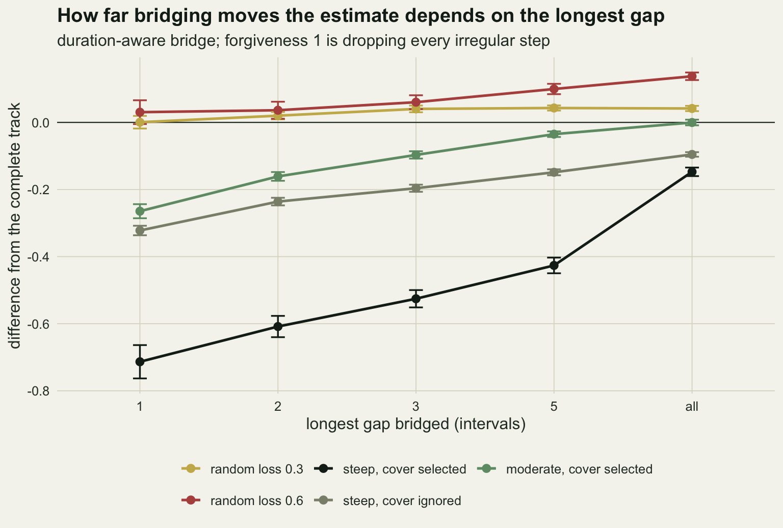
Under the steep model the difference from the complete track is -0.608 with a forgiveness of 2, -0.526 with 3, -0.426 with 5, and -0.147 (standard error 0.006) with every gap bridged. With every gap bridged it is -0.0003 (0.004) under the moderate model and -0.095 for the indifferent animal; the shorter forgiveness values are in the table and the figure. The one-kernel bridge, which bridges every gap, gives -0.385, -0.111 and -0.215.
A bridged step still ends at a fix that succeeded, so its end carries the same tilt by the fix probability as a regular step. What bridging adds is two things pulling the other way. The first is the upward lean of multi-interval steps from the section on why a longer step read as stronger selection. The second belongs to the loss itself: a step that spans three intervals exists because two fixes in a row failed, and fixes fail under cover, so the positions just before the end of a long bridged step were probably under cover, and on a smooth layer so was the end. The indifferent animal isolates the second pull, because with beta of 0 there is no selection for the first to amplify. Fitting the duration-aware model separately to the steps of each duration shows both, and random loss at 0.6 gives the baseline with no selective loss at all.
dur_tab <- do.call(rbind, lapply(c("r60", "st0", "st1", "md1"), function(k) {
  e <- settings[[k]]$est
  data.frame(setting = set_lab[[k]], duration = c("1", "2", "3 or more"),
             est = c(mean(e$dur_1), mean(e$dur_2), mean(e$dur_3)),
             se = c(sd(e$dur_1), sd(e$dur_2), sd(e$dur_3)) / sqrt(n_trk),
             full = mean(e$full), pooled = mean(e$cap_all), share_3 = mean(e$share_3))
}))
print(dur_tab, digits = 3, row.names = FALSE)
setting duration est se full pooled share_3
random loss 0.6 1 0.9966 0.01766 0.97294 1.1104 0.362
random loss 0.6 2 1.0328 0.02008 0.97294 1.1104 0.362
random loss 0.6 3 or more 1.2081 0.01480 0.97294 1.1104 0.362
steep, cover ignored 1 -0.3223 0.00834 0.00085 -0.0946 0.114
steep, cover ignored 2 -0.0163 0.01401 0.00085 -0.0946 0.114
steep, cover ignored 3 or more 0.3139 0.01205 0.00085 -0.0946 0.114
steep, cover selected 1 0.2044 0.02471 0.95365 0.8063 0.491
steep, cover selected 2 0.4916 0.02778 0.95365 0.8063 0.491
steep, cover selected 3 or more 1.0413 0.01127 0.95365 0.8063 0.491
moderate, cover selected 1 0.7121 0.01336 0.97074 0.9705 0.192
moderate, cover selected 2 0.9845 0.01825 0.97074 0.9705 0.192
moderate, cover selected 3 or more 1.4195 0.01535 0.97074 0.9705 0.192dv <- function(k, d) dur_tab$est[dur_tab$setting == set_lab[[k]] & dur_tab$duration == d]
dd <- function(k, v) mean(settings[[k]]$est[[v]] - settings[[k]]$est$full)
dd_se <- function(k, v) sd(settings[[k]]$est[[v]] - settings[[k]]$est$full) / sqrt(n_trk)
dur2_z <- (dd("r60", "dur_2") - thin_tab$diff[2]) / sqrt(dd_se("r60", "dur_2")^2 + thin_tab$se[2]^2)dur_tab$setting <- factor(dur_tab$setting, levels = set_lab[c("r60", "st0", "st1", "md1")])
ggplot(dur_tab, aes(duration, est)) +
geom_hline(aes(yintercept = full), linetype = "dashed", colour = te_ink, linewidth = 0.6) +
geom_hline(aes(yintercept = pooled), linetype = "dotted", colour = te_rust, linewidth = 0.9) +
geom_errorbar(aes(ymin = est - 2 * se, ymax = est + 2 * se), width = 0.12,
colour = te_forest, linewidth = 0.6) +
geom_point(size = 2.8, colour = te_forest) +
facet_wrap(~ setting, ncol = 2, scales = "free_y") +
labs(x = "step duration (intervals)", y = "cover coefficient",
title = "Short and long bridged steps disagree",
subtitle = "dashed: the complete track; dotted red: all durations pooled in one bridge") +
theme_datasheet() +
theme(strip.text = element_text(colour = te_ink, face = "bold"))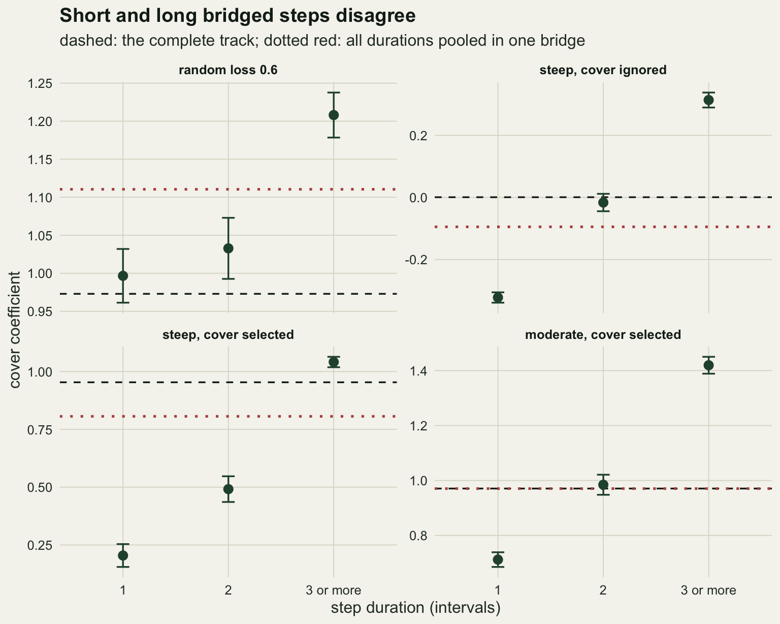
Under random loss the regular steps sit +0.024 from the complete track, the two-interval steps +0.060 and the steps of three intervals or more +0.235 (standard errors 0.011 to 0.018). The two-interval figure is 1.1 combined standard errors from the 0.080 of the thinned two-interval tracks, which it should match, since a bridged two-interval step under random loss is a two-interval displacement like any other. The duration classes disagree before any fix is lost selectively.
For the indifferent animal the regular steps say -0.322, the two-interval steps -0.016, and the steps of three intervals or more +0.314: taken alone, the long bridged steps report selection for cover that is not there. Under the steep model with beta of 1 the three are 0.204, 0.492 and 1.041, and the long steps are 49 per cent of all the steps in the bridge. Under the moderate model they are 0.712, 0.985 and 1.419, with long steps 19 per cent of the steps.
The pooled coefficient of the bridge is a compromise between these, and that is why it lands where it does. In the moderate setting it happens to land on the complete-track value, within its standard error; with the same model and the same layer it lands -0.147 away under the steep loss and +0.137 away under random loss of 0.6. Where a bridge ends up is set by the balance between the fix-probability tilt, the gap-length signal and the curvature of the layer, and none of the three is visible in the fitted model. The weights of the fix-loss post are the only arm here within two Monte Carlo standard errors of the complete track in every setting, and they need the fix model.
What to report
d_st1 <- sc_st1$est[c("ipw", "cap_all", "drop")] - sc_st1$est$full
rmse_one <- sqrt(colMeans(d_st1^2))
cross_n <- function(d) (var(d$ipw) - var(d$cap_all)) / (mean(d$cap_all)^2 - mean(d$ipw)^2)
n_star <- cross_n(d_st1)
n_star_boot <- apply(boot_i, 2, function(i) cross_n(d_st1[i, ]))
n_star_ci <- quantile(n_star_boot, c(0.025, 0.975))
print(round(c(rmse_one, n_star = n_star, n_star_ci), 3))
ipw cap_all drop n_star 2.5% 97.5%
0.369 0.163 0.763 6.116 4.278 9.916 Report the fix success of each collar and the share of steps that survive the regular-steps rule, and say whether fix success is known to depend on cover or terrain in the study area. If it does, the regular steps are biased in the direction of the fix-loss post, and bridging does not reliably remove that bias: it adds other biases that can offset it or not, and the pooled coefficient does not show which.
If a fix model is available from test collars, weight each stratum of the regular steps by one over the fix probability at the end of the step, and state the spread as well as the estimate. On a single track the weighted estimate is the noisier one: under the steep model the root mean square of its difference from the complete-track fit of the same track is 0.369, against 0.163 for the bridge with every gap bridged and 0.763 for the unweighted regular steps. The bridge’s error is mostly bias and does not average away; the weighted estimate’s error is mostly spread and does. Averaged over n independent tracks, the weighted estimate has the smaller mean squared error once n passes 6.1 in that setting. A bootstrap over the 120 tracks puts that crossover between 4.3 and 9.9 (2.5th and 97.5th percentiles over 2000 resamples), so it is a rough guide, not a threshold.
If gaps are bridged, report the forgiveness, the share of steps of each duration, and the cover coefficient fitted separately for each duration class. A disagreement between the classes is not by itself a sign of loss that follows cover: under random loss of 0.6 on this layer the two-interval steps sat +0.060 and the steps of three intervals or more +0.235 from the complete track, and none of that is loss. What a disagreement does show is that the pooled coefficient is a compromise between the classes rather than an estimate of any one of them. The drift that separates them was measured here on complete tracks, which a field study does not have.
Honest limits
Everything here comes from one cover layer made of three sine waves, one gamma movement kernel with no directional persistence, and 1500 steps per track. The upward lean of multi-interval steps is a property of the curvature of that layer at the scale of a bridged displacement; on a plane it vanished, on a rougher or smoother layer it would differ in size, and its sign on other layers is not measured here. Hofmann and colleagues, with two continuous layers and one binary layer of their own and fixes removed at random, found the habitat-selection estimates insensitive to the inclusion of irregular steps, and nothing here says their result is wrong for their design.
The weights use the true fix model at the true position. A field study estimates the fix model from stationary test collars, and the fix-loss post shows that an estimated model can do better or worse than no weighting depending on where the test collars stood. That error is not in this post and would add to the spread of the weighted arm.
Fixes fail independently given cover. Real failures cluster in time, when an animal beds under canopy or in a burrow, and clustering lengthens the gaps, which the forgiveness figure shows is exactly what moves the bridge. The weights assume independence too: with failures clustered in time, the probability that the end fix succeeds given that the start fix did is not the fix probability of the fix model, and the weight would need that conditional probability. Loss depends only on the covariate under study; time of day, terrain and collar orientation are not simulated.
The steep loss model leaves the selecting animal with only 21 per cent of its fixes, a severe case. The moderate model, with fix success running from 0.95 at a cover of -2 to 0.5 at a cover of 2, is a milder one, and it is the one in which the bridge happened to land on the complete track. Two cover-dependent models are two points on a continuum, and where along it the bridge crosses the complete track is not something a study could know without the fix model.
Each track is analysed alone, and the averages are over tracks of identical animals. No population model, random slopes or pooling across animals is run. Only the cover coefficient is examined. Hofmann and colleagues also assessed the movement-kernel parameters, which this post does not. Imputing the missing positions with a movement model, the approach of the track-regularising post, and bridging with composite paths stitched from one-interval steps are not run either.
The duration classes follow a rule fixed for this post: durations of five intervals or more share a kernel, and a class with fewer than 30 steps in a track joins the next shorter one. A study with a different rule would pool its long steps differently, and under cover-dependent loss the long steps are where the answer moves.
References
Hofmann DD, Cozzi G, Fieberg J 2024 Movement Ecology 12(1):37 (10.1186/s40462-024-00476-8)
Frair JL, Nielsen SE, Merrill EH, Lele SR, Boyce MS, Munro RHM, Stenhouse GB, Beyer HL 2004 Journal of Applied Ecology 41(2):201-212 (10.1111/j.0021-8901.2004.00902.x)
Fortin D, Beyer HL, Boyce MS, Smith DW, Duchesne T, Mao JS 2005 Ecology 86(5):1320-1330 (10.1890/04-0953)
Avgar T, Potts JR, Lewis MA, Boyce MS 2016 Methods in Ecology and Evolution 7(5):619-630 (10.1111/2041-210X.12528)
Horvitz DG, Thompson DJ 1952 Journal of the American Statistical Association 47(260):663-685 (10.1080/01621459.1952.10483446)