library(ggplot2)

te_pal <- list(forest = "#275139", green = "#2f8f63", sage = "#93a87f",
               clay = "#b5534e", gold = "#cda23f", line = "#dad9ca",
               ink = "#16241d", paper = "#f5f4ee")

theme_te <- function() {
  theme_minimal(base_size = 12) +
    theme(panel.grid.minor = element_blank(),
          panel.grid.major = element_line(colour = "#e7e6dc"),
          plot.background = element_rect(fill = "#f5f4ee", colour = NA),
          panel.background = element_rect(fill = "#f5f4ee", colour = NA),
          plot.title = element_text(face = "bold", colour = te_pal$ink),
          axis.title = element_text(colour = "#2c3a31"),
          axis.text = element_text(colour = "#2c3a31"))
}Transporting an effect to a new region
R
causal inference
transportability
external validity
ecology tutorial
An effect measured in one valley is wanted for a whole region. Measuring the sign flip, the transport formula, the precision it costs and the two failures.
A grazing exclusion trial in one valley: three hundred and twenty permanent plots on semi-natural grassland, each either fenced against sheep or left open, with vascular plant richness recorded in a four square metre quadrat after six seasons. The plots were not fenced at random. The wetter ground at the valley floor was easier to secure and got fenced more often than the dry upper slopes, so soil moisture drives both the treatment and the outcome, and the raw comparison is confounded. Soil moisture was measured on every plot, so the confounding is the kind that adjustment handles.
The result goes into a report, and the report is read by an agency that regulates grazing across the whole upland district: forty thousand mapped grassland parcels, moisture known for every one of them from a soil survey and a wetness index, and no outcome data anywhere except in that one valley. The question the agency asks is not the one the trial answered. The trial answered what fencing did to the plots in the valley; the agency wants to know what a district-wide prescription would do to the district.
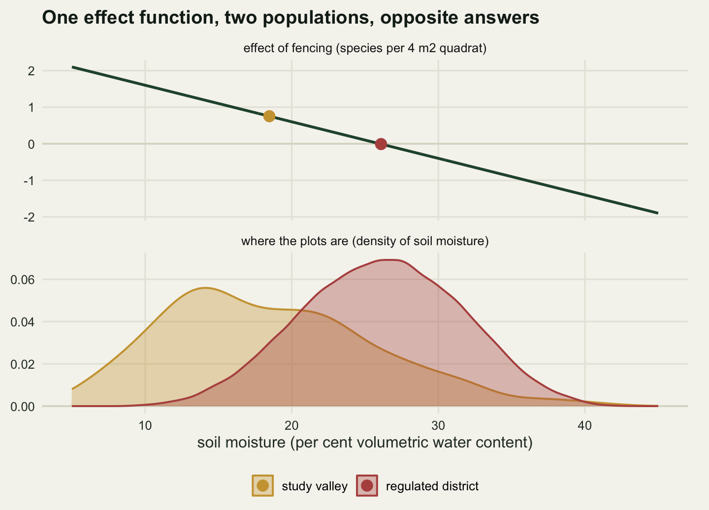
Those two numbers are not the same, and the gap is not sampling error. Herbivore removal does different things on different ground: Bakker et al (2006) found across grasslands that grazing raises plant diversity where habitats are productive and lowers it where they are not, so the sign of a grazing effect depends on where you stand. The study valley is dry, and the district includes a great deal of wet, productive ground that the valley barely represents. Averaging one effect function over two different moisture distributions gives two different answers, and the difference can be larger than the effect.
This post is positioned directly against G-computation and standardisation. That post fits an outcome model, predicts the potential outcome for every unit under each treatment level, averages, and takes the difference. Its own code names the target in a comment: the true SAMPLE-marginal effect. The averaging runs over the covariate distribution of the sample in hand, which is right if that sample is the population you care about, and nothing there asks whether it is. Here the machinery is nearly identical and one thing changes: the averaging runs over a different population’s covariate distribution. The arithmetic is a line of code apart. The assumption behind it is not, and that assumption has no test.
The other neighbour is Checking causal assumptions, which stresses the internal-validity premise with negative controls and a robustness value. Everything it checks is about whether the estimate is right for the units that were studied. Nothing in it, and nothing else in this blog’s causal cluster, asks whether those units are the units the decision is about. That second question is what follows.
Six things get measured: the effect in the valley, what the valley’s interval covers when the district is the target, the transport formula run two ways, the precision it costs, a diagnostic that warns early, and two ways the whole thing fails while looking healthy.
Two populations, one effect function
The generating model has one covariate doing three jobs. Soil moisture confounds, because it drives fencing; it is prognostic, because wetter grassland carries more species anyway; and it modifies, because the sign of the fencing effect depends on it. Write \(W\) for moisture as per cent volumetric water content, \(A\) for the fencing indicator and \(Y\) for richness in the quadrat:
\[E[Y \mid A, W] = \mu(W) + \tau(W)\,A, \qquad \tau(W) = \tau_0 + \tau_1 W\]
The single decision that makes transport possible is that \(\tau(\cdot)\) is the same function in the valley and in the district: two plots with the same soil moisture respond to fencing the same way, wherever they are. That is the transportability assumption in full, and the simulation is built so that it holds. What differs between the two places is only the distribution of \(W\).
w_lo <- 4; w_hi <- 46; n_study <- 320; n_target <- 40000; sd_noise <- 1.6
tau_0 <- 2.6; tau_1 <- -0.10; zero_at <- -tau_0 / tau_1

tau_of <- function(w) tau_0 + tau_1 * w
mu_of <- function(w) 9 + 0.22 * w
prop_of <- function(w) 1 / (1 + exp(-(-0.4 + 0.08 * (w - 18))))
set.seed(20260802)
w_target <- w_lo + (w_hi - w_lo) * rbeta(n_target, 7.235, 6.515)

study_of <- function(seed) {
  set.seed(seed)
  w <- w_lo + (w_hi - w_lo) * rbeta(n_study, 2.2, 4.4)
  a <- rbinom(n_study, 1, prop_of(w))
  data.frame(y = mu_of(w) + tau_of(w) * a + rnorm(n_study, 0, sd_noise),
             a = a, w = w)
}
d_val <- study_of(20260803)
truth_val <- mean(tau_of(d_val$w))
truth_tgt <- mean(tau_of(w_target))
print(round(c(plots = n_study, fenced = sum(d_val$a), parcels = n_target,
              valley_mean = mean(d_val$w), valley_sd = sd(d_val$w),
              valley_min = min(d_val$w), valley_max = max(d_val$w)), 3))
plots fenced parcels valley_mean valley_sd valley_min
320.000 137.000 40000.000 18.468 7.115 4.980
valley_max
41.145 print(round(c(district_mean = mean(w_target), district_sd = sd(w_target),
district_min = min(w_target), district_max = max(w_target),
propensity_min = min(prop_of(d_val$w)),
propensity_max = max(prop_of(d_val$w))), 3)) district_mean district_sd district_min district_max propensity_min
26.091 5.450 8.817 43.155 0.191
propensity_max
0.810 print(round(c(zero_effect_moisture = zero_at, truth_valley = truth_val,
truth_district = truth_tgt), 4))zero_effect_moisture truth_valley truth_district
26.0000 0.7532 -0.0091 The valley averages 18.47 per cent moisture with a standard deviation of 7.11; the district averages 26.09 per cent with a standard deviation of 5.45. Both sit inside the same physical range, so this is not yet a story about the district holding conditions the valley has never seen; that case comes later. It is a story about the same conditions mixed in different proportions.
The effect function crosses zero at 26 per cent moisture. Below that, fencing adds species; above it, fencing removes them, the ungrazed sward closing over and the small forbs going out. Average \(\tau(W)\) over the valley’s 320 plots and the answer is 0.7532 species per quadrat. Average the same function over the district’s 40000 parcels and the answer is -0.0091. One number says fencing gains most of a species per quadrat; the other says fencing does nothing at all. Neither is wrong. They are averages of one function over two different populations.
The fencing propensity runs from 0.191 on the driest plot to 0.81 on the wettest, so both treatments are possible everywhere in the valley and internal positivity is comfortable. The failures measured later are not positivity failures inside the study; they are failures of a different condition that looks similar.
The valley answer, done properly
Standardisation on the study data is the g-computation post’s procedure without a comma changed. Fit an outcome model that allows the effect to depend on moisture, predict every plot’s richness twice, once with the fence and once without, and take the mean difference.
gcomp <- function(fit, newdat) {
  mean(predict(fit, transform(newdat, a = 1)) -
         predict(fit, transform(newdat, a = 0)))
}

se_marg <- function(fit, wbar, extra = 0) {
  kv <- setNames(rep(0, length(coef(fit))), names(coef(fit)))
  kv["a"] <- 1; kv["a:w"] <- wbar
  sqrt(drop(t(kv) %*% vcov(fit) %*% kv) + extra)
}
fit_val <- lm(y ~ a * w, data = d_val)
naive_val <- mean(d_val$y[d_val$a == 1]) - mean(d_val$y[d_val$a == 0])
est_val <- gcomp(fit_val, d_val)
se_val <- se_marg(fit_val, mean(d_val$w),
                  unname(coef(fit_val)["a:w"])^2 * var(d_val$w) / n_study)
ci_val <- est_val + c(-1, 1) * qt(0.975, df.residual(fit_val)) * se_val
print(round(summary(fit_val)$coefficients, 4))
Estimate Std. Error t value Pr(>|t|)
(Intercept) 9.0379 0.3183 28.3964 0
a 3.1083 0.5014 6.1993 0
w 0.2151 0.0178 12.1123 0
a:w -0.1233 0.0250 -4.9357 0print(round(c(naive_difference = naive_val, standardised_valley = est_val,
se = se_val, lower = ci_val[1], upper = ci_val[2],
valley_truth = truth_val), 4)) naive_difference standardised_valley se lower
1.4069 0.8302 0.1861 0.4641
upper valley_truth
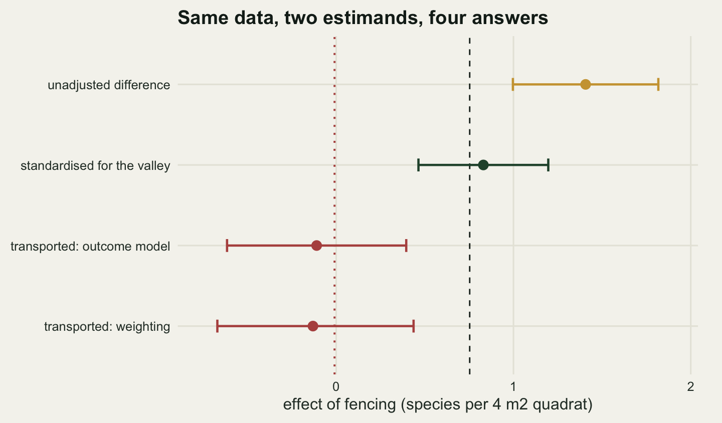
1.1964 0.7532 The unadjusted difference between fenced and open plots is 1.4069 species, nearly twice the truth. The confounding runs through the main effect: fenced plots are the wet ones, wet grassland carries more species whatever is done to it, and the raw comparison charges that baseline difference to the fence. Standardisation returns 0.8302 species with an interval of 0.4641 to 1.1964, covering the valley truth of 0.7532.
Two details in the standard error recur below. The estimator is a linear combination of the fitted coefficients, \(\hat\beta_A + \hat\beta_{AW}\bar{W}\), so its variance follows from the coefficient covariance without a bootstrap; and because the valley’s own mean moisture is estimated from 320 plots, the valley version carries an extra term \(\hat\beta_{AW}^2 \operatorname{Var}(\bar W)\) that the district does not, the district’s mean being a census figure over 40000 parcels.
One dataset settles nothing, so the procedure runs over many valleys. Each replicate redraws the plots, the fencing and the noise, refits, and records the estimate, its interval and the valley truth for that draw.
n_rep <- 500
rep_tab <- matrix(NA_real_, n_rep, 5)
for (b in seq_len(n_rep)) {
  db <- study_of(41000 + b)
  fb <- lm(y ~ a * w, data = db)
  rep_tab[b, ] <- c(
    gcomp(fb, db),
    se_marg(fb, mean(db$w), unname(coef(fb)["a:w"])^2 * var(db$w) / n_study),
    gcomp(fb, data.frame(w = w_target)),
    se_marg(fb, mean(w_target)), mean(tau_of(db$w)))
}
colnames(rep_tab) <- c("est_v", "se_v", "est_t", "se_t", "truth_v")
rep_tab <- as.data.frame(rep_tab)

t_crit <- qt(0.975, n_study - 4)
cov_own <- mean(abs(rep_tab$est_v - rep_tab$truth_v) < t_crit * rep_tab$se_v)
cov_wrong <- mean(abs(rep_tab$est_v - truth_tgt) < t_crit * rep_tab$se_v)
bias_val <- mean(rep_tab$est_v - rep_tab$truth_v)
mc_val <- sd(rep_tab$est_v - rep_tab$truth_v) / sqrt(n_rep)
print(round(c(replicates = n_rep, mean_estimate = mean(rep_tab$est_v),
              mean_valley_truth = mean(rep_tab$truth_v),
              bias = bias_val, mc_se_of_bias = mc_val,
              coverage_of_valley_truth = cov_own,
              coverage_of_district_truth = cov_wrong,
              mean_se = mean(rep_tab$se_v),
              sd_of_estimates = sd(rep_tab$est_v)), 5))
replicates mean_estimate
500.00000 0.81262
mean_valley_truth bias
0.79984 0.01278
mc_se_of_bias coverage_of_valley_truth
0.00878 0.94000
coverage_of_district_truth mean_se
0.01400 0.19511
sd_of_estimates
0.19759 Over 500 replicates the standardised estimate averages 0.8126 against a mean valley truth of 0.7998, a bias of 0.01278 with a Monte Carlo standard error of 0.00878, and the interval covers the valley truth 94 per cent of the time. The model form is correct, the confounder is measured, positivity holds, and the answer is unbiased with nominal coverage.
What that interval covers, and what it does not
The same numbers read against the other target tell a different story. Nothing about the estimator changes; only the question does.
gap_val <- truth_val - truth_tgt
gap_in_se <- (mean(rep_tab$est_v) - truth_tgt) / mean(rep_tab$se_v)
nearest_edge <- min(abs(rep_tab$est_v - t_crit * rep_tab$se_v - truth_tgt))
print(round(c(valley_truth = truth_val, district_truth = truth_tgt,
              gap = gap_val, gap_in_standard_errors = gap_in_se,
              coverage_of_district_truth = cov_wrong,
              replicates_covering = round(cov_wrong * n_rep),
              closest_approach_of_lower_limit = nearest_edge), 4))
valley_truth district_truth
0.7532 -0.0091
gap gap_in_standard_errors
0.7623 4.2117
coverage_of_district_truth replicates_covering
0.0140 7.0000
closest_approach_of_lower_limit
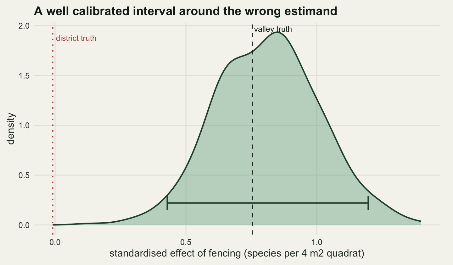
0.0021 The valley interval contains the district truth in 1.4 per cent of replicates, 7 out of 500. The estimate sits 4.212 standard errors from the quantity the agency will act on, and the smallest gap in either direction between that quantity and a replicate’s lower limit was 0.0021 species.
This is a confident, well calibrated interval around the wrong estimand. Every diagnostic an analyst would reach for is clean, because nothing is wrong with the model: residuals fine, coverage nominal for the quantity estimated, confounding handled, a negative control null. The failure is in the sentence written under the fit, which silently swaps the population the average was taken over for the population the reader has in mind. No statistic sees that swap, because it happens in the prose.
The transport formula
The repair is one substitution. Standardisation averages the predicted contrast over a covariate distribution; supply the district’s distribution instead of the valley’s. Written out, with \(P\) the study population and \(Q\) the target,
\[\hat\tau_Q \;=\; \frac{1}{n_Q}\sum_{i \in Q}\Big[\hat{m}(1, W_i) - \hat{m}(0, W_i)\Big]\]
where \(\hat{m}\) is the outcome model fitted on the study data alone. It never sees a district outcome, because there are none; it sees 40000 district moisture values and predicts into them. This is the outcome-model route, and it is the object Pearl and Bareinboim (2014) obtain from their selection diagrams when the difference between populations is confined to the distribution of a measured modifier.
A second route never predicts anything. Reweight the study plots so that their moisture distribution matches the district’s, then estimate the effect in the reweighted sample. The weight is the density ratio \(f_Q(W)/f_P(W)\), estimated by pooling the study plots with a sample of district parcels, fitting a model for which population a unit came from, and taking the odds. Cole and Stuart (2010) introduced this for taking a clinical trial to a national target population, and Westreich et al (2017) set out the same weight as inverse odds of sampling weights; Stuart et al (2011) use the participation model as a diagnostic for how far apart two populations are before any estimate is attempted.
est_out <- gcomp(fit_val, data.frame(w = w_target))
se_out <- se_marg(fit_val, mean(w_target))
ci_out <- est_out + c(-1, 1) * qt(0.975, df.residual(fit_val)) * se_out
n_pool <- 2000
set.seed(77001)
w_pool <- sample(w_target, n_pool)

ratio_of <- function(dstudy, wpop) {
  pooled <- data.frame(w = c(dstudy$w, wpop),
                       s = c(rep(1L, nrow(dstudy)), rep(0L, length(wpop))))
  m_part <- suppressWarnings(glm(s ~ w + I(w^2), binomial, pooled))
  p_in <- predict(m_part, data.frame(w = dstudy$w), type = "response")
  ((1 - p_in) / p_in) * (nrow(dstudy) / length(wpop))
}

hajek <- function(dstudy, e_hat, wt) {
  a1 <- dstudy$a == 1; a0 <- !a1
  sum(wt[a1] * dstudy$y[a1] / e_hat[a1]) / sum(wt[a1] / e_hat[a1]) -
    sum(wt[a0] * dstudy$y[a0] / (1 - e_hat[a0])) /
    sum(wt[a0] / (1 - e_hat[a0]))
}
dens_ratio <- ratio_of(d_val, w_pool)
e_val <- fitted(glm(a ~ w, family = binomial, data = d_val))
est_wt <- hajek(d_val, e_val, dens_ratio)
set.seed(77002)
n_boot <- 600
boot_wt <- numeric(n_boot)
for (b in seq_len(n_boot)) {
  db <- d_val[sample.int(n_study, n_study, replace = TRUE), ]
  eb <- fitted(suppressWarnings(glm(a ~ w, binomial, db)))
  boot_wt[b] <- hajek(db, eb, ratio_of(db, w_pool))
}
ci_wt <- unname(quantile(boot_wt, c(0.025, 0.975)))
print(round(c(valley_standardised = est_val,
              transported_outcome_model = est_out,
              transported_weighting = est_wt, district_truth = truth_tgt), 4))
valley_standardised transported_outcome_model transported_weighting
0.8302 -0.1101 -0.1309
district_truth
-0.0091 print(round(c(se_outcome = se_out, lower_outcome = ci_out[1],
upper_outcome = ci_out[2], se_weighting = sd(boot_wt),
lower_weighting = ci_wt[1], upper_weighting = ci_wt[2]), 4)) se_outcome lower_outcome upper_outcome se_weighting lower_weighting
0.2568 -0.6154 0.3953 0.2896 -0.6701
upper_weighting
0.4366 On this valley the outcome-model transport returns -0.1101 species with an interval of -0.6154 to 0.3953, and the weighting route returns -0.1309 with a bootstrap interval of -0.6701 to 0.4366. Both cover the district truth of -0.0091, and both sit a long way from the 0.8302 the same data gave for the valley. Two estimators, one built on the outcome model and one on a pair of propensity-style models, land in the same place.
The weighting route is wider here, its standard error 0.2896 against 0.2568, which is the usual ordering: it throws away the parametric structure the outcome model exploits. Dahabreh et al (2020) set out both kinds together with the augmented combination that the AIPW tutorial builds in the internal-validity setting, which here would buy the same insurance from the same two models. Whether transport is unbiased, rather than lucky on one valley, is the question already asked of standardisation, and the replicate loop stored the answer.
cov_trans <- mean(abs(rep_tab$est_t - truth_tgt) < t_crit * rep_tab$se_t)
bias_trans <- mean(rep_tab$est_t) - truth_tgt
mc_trans <- sd(rep_tab$est_t) / sqrt(n_rep)
se_price <- mean(rep_tab$se_t) / mean(rep_tab$se_v)
print(c(mean_transported = formatC(mean(rep_tab$est_t), format = "f", digits = 5),
        district_truth = formatC(truth_tgt, format = "f", digits = 5),
        bias = formatC(bias_trans, format = "f", digits = 5),
        mc_se_of_mean = formatC(mc_trans, format = "f", digits = 5)))
mean_transported district_truth bias mc_se_of_mean
"-0.00005" "-0.00913" "0.00908" "0.01285" print(round(c(coverage_of_district_truth = cov_trans,
mean_se_valley = mean(rep_tab$se_v),
mean_se_transported = mean(rep_tab$se_t), se_ratio = se_price,
sd_ratio = sd(rep_tab$est_t) / sd(rep_tab$est_v)), 4))coverage_of_district_truth mean_se_valley
0.9320 0.1951
mean_se_transported se_ratio
0.2755 1.4120
sd_ratio
1.4545 Over the same 500 replicates the transported estimate averages -0.00005 against a district truth of -0.00913, a bias of 0.00908 with a Monte Carlo standard error of 0.01285, which is to say no measurable bias at this number of replicates. Coverage of the district truth is 93.2 per cent, against the 1.4 per cent the untransported interval managed.
The price
Transport is not free, and the bill arrives in the standard error.
lev_gap <- (mean(w_target) - mean(d_val$w)) / sd(d_val$w)
width_gain <- 100 * (se_price - 1)
n_equiv <- n_study / se_price^2
print(round(c(valley_mean_moisture = mean(d_val$w),
              district_mean_moisture = mean(w_target),
              gap_in_valley_sd_units = lev_gap, se_ratio = se_price,
              per_cent_wider = width_gain, plots_equivalent_to = n_equiv,
              plots_actual = n_study,
              plots_thrown_away = n_study - n_equiv), 3))
valley_mean_moisture district_mean_moisture gap_in_valley_sd_units
18.468 26.091 1.071
se_ratio per_cent_wider plots_equivalent_to
1.412 41.198 160.506
plots_actual plots_thrown_away
320.000 159.494 The transported standard error is 1.412 times the valley one, so the interval is 41.2 per cent wider. The reason is geometric. The estimator is \(\hat\beta_A + \hat\beta_{AW}\bar{W}\), and the variance of that combination is smallest when \(\bar{W}\) sits at the centre of the study’s own moisture distribution and grows as it moves away. The district’s mean sits 1.071 valley standard deviations from the valley’s mean, and the study data is thin out there: the plots that carry information about the effect on wet ground are the handful of plots that happened to be wet.
Read in units the field crew would recognise, an interval 1.412 times wider is what 161 plots would have given at the valley’s own target. The trial has 320. Transporting the answer costs the equivalent of 159 plots, spent not on measuring anything but on aiming the estimate somewhere the design was not centred.
A diagnostic that fires before the interval does
The density ratio is worth looking at for its own sake, because it is the only part of the procedure that speaks about the two populations rather than about one model. A weighted average with unequal weights behaves like a smaller sample, and the standard measure of how much smaller is the effective sample size,
\[n_{\text{eff}} = \frac{\left(\sum_i w_i\right)^2}{\sum_i w_i^2}\]
which equals the sample size when all weights are equal and falls towards one as a single plot takes over.
ess_of <- function(wt) sum(wt)^2 / sum(wt^2)
# a second, wetter candidate target, used from here on as a contrast
set.seed(20260806)
w_wet <- w_lo + (w_hi - w_lo) * rbeta(n_target, 12, 4)
set.seed(77003)
w_pool_wet <- sample(w_wet, n_pool)
ess_main <- ess_of(dens_ratio)
share_main <- max(dens_ratio) / sum(dens_ratio)
top10_main <- sum(sort(dens_ratio, decreasing = TRUE)[1:10]) / sum(dens_ratio)
print(round(c(plots = n_study, effective_sample_size = ess_main,
              per_cent_of_plots = 100 * ess_main / n_study,
              largest_weight = max(dens_ratio),
              largest_weight_share_pct = 100 * share_main,
              top_ten_share_pct = 100 * top10_main,
              se_ratio_measured = se_price), 3))
plots effective_sample_size per_cent_of_plots
320.000 143.950 44.985
largest_weight largest_weight_share_pct top_ten_share_pct
3.537 1.116 11.145
se_ratio_measured
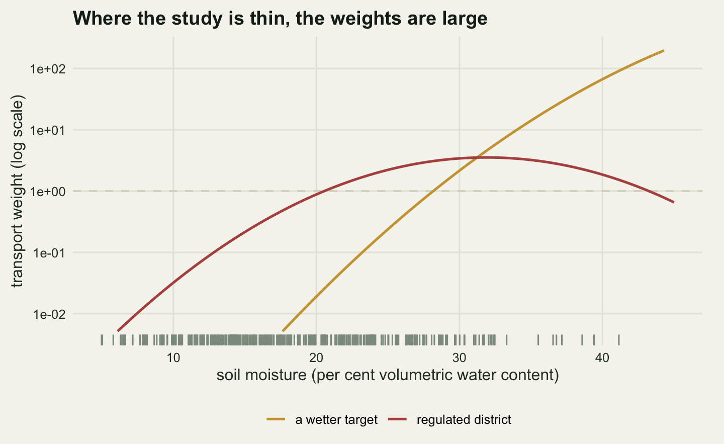
1.412 The transport weights have an effective sample size of 144 plots out of 320, 45 per cent of the sample. The largest single weight takes 1.12 per cent of the total and the ten largest take 11.14 per cent, so no one plot is running the show. That agrees with what the standard error did: an effective sample size of 45 per cent and a standard error ratio of 1.412 are two views of one loss of information. The diagnostic can be computed before any outcome is used, from the study covariates and the target covariates alone, so a team that runs it at the design stage learns how much of its sample will survive the journey and can still move plots.
An effect modifier nobody measured
Everything so far worked because soil moisture was the whole story: the only thing that modified the effect, and measured in both places. Drop either half of that and the transport formula returns a number with the same shape and none of the meaning.
Suppose a second modifier exists. Soil phosphorus varies within the valley, and the fencing effect falls as phosphorus rises, the extra fertility feeding the tall grasses that shade the forbs out once grazing stops. Phosphorus is not a confounder here: it has nothing to do with which plots got fenced, so leaving it out of the model costs the valley estimate nothing. But the district lies on a different parent material and is markedly richer in phosphorus, and nobody has mapped it.
p_shift <- 1.2
p_slope <- -0.55

study_p <- function(seed) {
  set.seed(seed)
  w <- w_lo + (w_hi - w_lo) * rbeta(n_study, 2.2, 4.4)
  phos <- rnorm(n_study, 0, 1)
  a <- rbinom(n_study, 1, prop_of(w))
  y <- mu_of(w) + 0.5 * phos + (tau_of(w) + p_slope * phos) * a +
    rnorm(n_study, 0, sd_noise)
  data.frame(y = y, a = a, w = w, phos = phos)
}
truth_tgt_p <- truth_tgt + p_slope * p_shift
n_rep_p <- 400
rep_p <- matrix(NA_real_, n_rep_p, 4)
for (b in seq_len(n_rep_p)) {
  db <- study_p(52000 + b)
  fb <- lm(y ~ a * w, data = db)
  rep_p[b, ] <- c(gcomp(fb, data.frame(w = w_target)),
                  se_marg(fb, mean(w_target)), gcomp(fb, db),
                  mean(tau_of(db$w) + p_slope * db$phos))
}
colnames(rep_p) <- c("est_t", "se_t", "est_v", "truth_v")
rep_p <- as.data.frame(rep_p)

cov_p <- mean(abs(rep_p$est_t - truth_tgt_p) < t_crit * rep_p$se_t)
bias_p <- mean(rep_p$est_t) - truth_tgt_p
half_p <- t_crit * mean(rep_p$se_t)
correction <- truth_val - truth_tgt
print(round(c(district_truth_with_phosphorus = truth_tgt_p,
              transported_estimate = mean(rep_p$est_t), bias = bias_p,
              mc_se = sd(rep_p$est_t) / sqrt(n_rep_p),
              coverage_of_district_truth = cov_p,
              mean_interval_half_width = half_p,
              bias_over_half_width = bias_p / half_p), 4))
district_truth_with_phosphorus transported_estimate
-0.6691 0.0130
bias mc_se
0.6822 0.0137
coverage_of_district_truth mean_interval_half_width
0.3150 0.5592
bias_over_half_width
1.2198 print(round(c(valley_estimate = mean(rep_p$est_v),
valley_truth = mean(rep_p$truth_v),
correction_transport_made = correction,
error_it_left_behind = bias_p,
error_as_share_of_correction = bias_p / correction), 4)) valley_estimate valley_truth
0.8147 0.8001
correction_transport_made error_it_left_behind
0.7623 0.6822
error_as_share_of_correction
0.8949 The district runs 1.2 standard deviations higher in phosphorus than the valley, and the fencing effect falls by 0.55 species per standard deviation of it. The transported estimate averages 0.013 species over 400 replicates, against a district truth that is now -0.6691. The bias is 0.6822, the interval covers the truth 31.5 per cent of the time, and the interval itself has not changed shape at all: its half width is 0.5592, essentially what it was in the working case. The valley estimate is still fine, averaging 0.8147 against a valley truth of 0.8001, because phosphorus is balanced across fencing within the valley and its omission costs nothing there.
Put the two numbers side by side. Transporting moved the estimate 0.7623 species, from the valley average to the district average, and the error left behind by the unmeasured modifier is 0.6822 species, 89.5 per cent of the correction just made. The procedure travelled most of the distance, stopped, and gave no indication of where. Catford et al (2022) make the general version of this point: context dependence is not noise to be averaged away but a set of specific moderators, and a claim that travels is a claim about which moderators were captured.
There is no test for this. The valley data hold no information about a variable never measured, and the district data hold no outcomes at all. The only defence is subject knowledge: list what plausibly changes the sign or size of the effect, and check that each item is measured in both populations. A modifier that fails the check does not make transport impossible; it makes the transported number conditional on that modifier being similarly distributed, a claim to be argued rather than computed.
Where the target leaves the study behind
The second failure is different in kind. So far both populations occupied the same range of soil moisture and only their proportions differed. Now the target is a wetter district, averaging 35.5 per cent moisture, with a substantial share of parcels above anything the valley contains.
hinge_at <- 30
sup_hi <- unname(quantile(d_val$w, 0.99))
frac_in_main <- mean(w_target <= sup_hi)
frac_in_wet <- mean(w_wet <= sup_hi)
frac_above_max <- mean(w_wet > max(d_val$w))

dens_wet <- ratio_of(d_val, w_pool_wet)
ess_wet <- ess_of(dens_wet)
share_wet <- max(dens_wet) / sum(dens_wet)
print(round(c(valley_max = max(d_val$w), valley_99th = sup_hi,
              wet_target_mean = mean(w_wet), wet_target_max = max(w_wet),
              share_of_wet_target_inside = frac_in_wet,
              share_of_wet_above_valley_max = frac_above_max,
              share_of_district_inside = frac_in_main), 4))
valley_max valley_99th
41.1445 37.0883
wet_target_mean wet_target_max
35.4947 45.4707
share_of_wet_target_inside share_of_wet_above_valley_max
0.6031 0.0846
share_of_district_inside
0.9828 print(round(c(ess_district = ess_main, ess_wet_target = ess_wet,
ess_wet_as_pct_of_plots = 100 * ess_wet / n_study,
largest_weight_district = max(dens_ratio),
largest_weight_wet = max(dens_wet),
largest_share_wet_pct = 100 * share_wet), 3)) ess_district ess_wet_target ess_wet_as_pct_of_plots
143.950 9.377 2.930
largest_weight_district largest_weight_wet largest_share_wet_pct
3.537 91.172 23.419 The diagnostics fire loudly. Only 60.3 per cent of the wetter target lies below the valley’s ninety-ninth percentile, against 98.3 per cent for the district used earlier, and 8.5 per cent of it lies above the wettest plot the trial ever measured. The effective sample size of the transport weights collapses from 144 plots to 9.4, or 2.9 per cent of the sample, and one plot now carries 23.4 per cent of the total weight against 1.12 per cent before. A weighting estimator built on that is effectively an experiment with 9 plots in it.
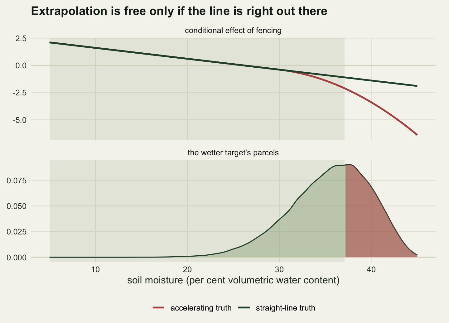
The outcome-model route does not collapse in the same visible way, and that is what makes it dangerous. It will happily predict at 45.5 per cent moisture, the wettest parcel in the target, because a fitted line has a value everywhere. Whether that value is right depends on whether the effect function really is the straight line the model assumed, out where no plot ever was, and the study data cannot settle it. Two truths, identical inside the valley’s range and different outside it: the straight line used so far, and one where the fencing penalty accelerates once the ground is waterlogged past 30 per cent moisture.
tau_hinge <- function(w) tau_of(w) - 0.02 * pmax(w - hinge_at, 0)^2

study_h <- function(seed, tfun) {
  set.seed(seed)
  w <- w_lo + (w_hi - w_lo) * rbeta(n_study, 2.2, 4.4)
  a <- rbinom(n_study, 1, prop_of(w))
  data.frame(y = mu_of(w) + tfun(w) * a + rnorm(n_study, 0, sd_noise),
             a = a, w = w)
}
n_rep_o <- 400
rep_o <- matrix(NA_real_, n_rep_o, 9)
for (b in seq_len(n_rep_o)) {
  d_lin <- study_h(63000 + b, tau_of)
  d_hin <- study_h(63000 + b, tau_hinge)
  f_lin <- lm(y ~ a * w, data = d_lin)
  f_hin <- lm(y ~ a * w, data = d_hin)
  keep <- w_wet <= unname(quantile(d_hin$w, 0.99))
  rep_o[b, ] <- c(gcomp(f_lin, data.frame(w = w_wet)),
                  se_marg(f_lin, mean(w_wet)),
                  gcomp(f_hin, data.frame(w = w_wet)),
                  se_marg(f_hin, mean(w_wet)),
                  gcomp(f_hin, data.frame(w = w_wet[keep])),
                  se_marg(f_hin, mean(w_wet[keep])),
                  mean(tau_hinge(w_wet[keep])), mean(keep),
                  gcomp(f_hin, d_hin) - mean(tau_hinge(d_hin$w)))
}
colnames(rep_o) <- c("lin", "lin_se", "hin", "hin_se", "res", "res_se",
                     "res_truth", "covered", "in_sample_bias")
rep_o <- as.data.frame(rep_o)

truth_wet_lin <- mean(tau_of(w_wet))
truth_wet_hin <- mean(tau_hinge(w_wet))
cov_lin <- mean(abs(rep_o$lin - truth_wet_lin) < t_crit * rep_o$lin_se)
cov_hin <- mean(abs(rep_o$hin - truth_wet_hin) < t_crit * rep_o$hin_se)
bias_hin <- mean(rep_o$hin) - truth_wet_hin
print(round(c(wet_truth_straight_line = truth_wet_lin,
              estimate_straight_line = mean(rep_o$lin),
              bias_straight_line = mean(rep_o$lin) - truth_wet_lin,
              coverage_straight_line = cov_lin), 4))
wet_truth_straight_line estimate_straight_line bias_straight_line
-0.9495 -0.9438 0.0057
coverage_straight_line
0.9550 print(round(c(wet_truth_accelerating = truth_wet_hin,
estimate_accelerating = mean(rep_o$hin),
bias_accelerating = bias_hin,
coverage_accelerating = cov_hin,
mean_se_straight = mean(rep_o$lin_se),
mean_se_accelerating = mean(rep_o$hin_se),
in_sample_bias = mean(rep_o$in_sample_bias)), 4))wet_truth_accelerating estimate_accelerating bias_accelerating
-1.9111 -1.1588 0.7523
coverage_accelerating mean_se_straight mean_se_accelerating
0.6525 0.4843 0.4855
in_sample_bias
0.0065 Under the straight-line truth, transport to the wetter target is unbiased: -0.9438 against -0.9495, coverage 95.5 per cent, even though 8.5 per cent of the target is outside the study’s observed range. Extrapolation into a region the data never saw is free when the assumed functional form happens to be correct there.
Under the accelerating truth it is not free. The estimate averages -1.1588 against a truth of -1.9111, a bias of 0.7523 species, and coverage drops to 65.25 per cent. The two cases have standard errors of 0.4843 and 0.4855, effectively the same, and identical overlap diagnostics, those being functions of the covariates only. Within the valley the curvature is invisible: the standardised valley estimate under it is biased by 0.0065 species, only a handful of plots being wet enough to show it.
The honest response is to stop extrapolating and say so: restrict the target to the region of common support, report the effect there, and report what fraction of the target it covers.
cov_res <- mean(abs(rep_o$res - rep_o$res_truth) < t_crit * rep_o$res_se)
bias_res <- mean(rep_o$res - rep_o$res_truth)
print(round(c(share_of_wet_target_covered = mean(rep_o$covered),
              sd_of_that_share = sd(rep_o$covered),
              share_using_this_valley = frac_in_wet,
              restricted_estimate = mean(rep_o$res),
              restricted_truth = mean(rep_o$res_truth),
              bias = bias_res, coverage = cov_res), 4))
share_of_wet_target_covered sd_of_that_share
0.4635 0.1036
share_using_this_valley restricted_estimate
0.6031 -0.7290
restricted_truth bias
-0.7546 0.0257
coverage
0.9525 print(round(c(whole_target_truth = truth_wet_hin,
whole_target_estimate = mean(rep_o$hin),
restricted_truth = mean(rep_o$res_truth),
understatement = mean(rep_o$res_truth) - truth_wet_hin), 4)) whole_target_truth whole_target_estimate restricted_truth
-1.9111 -1.1588 -0.7546
understatement
1.1565 Restricted to the parcels below the valley’s ninety-ninth percentile of moisture, which is 46.4 per cent of the wetter target, the transported estimate is -0.729 against a restricted truth of -0.7546, a bias of 0.0257 with 95.25 per cent coverage. The estimator works again, because the question shrank to fit the data.
How far it shrank is itself uncertain. The covered share averages 46.4 per cent across replicate valleys with a standard deviation of 10.4 percentage points, against 60.3 per cent for the valley used above. The common-support boundary is a ninety-ninth percentile of 320 plots, so the size of the region a study can honestly speak for is itself a statistic with a standard error.
That shrinkage is the cost, and it should be reported rather than buried. The restricted answer, -0.7546 species, understates the whole-target effect of -1.9111 by 1.1565 species, because the parcels left out are exactly the ones where fencing does most harm. A regulator reading only the restricted number would underestimate the damage; a regulator reading only the extrapolated number would get a figure 39.4 per cent off with an interval that does not admit it. The choice between them is not statistical. It is a choice about which kind of error the decision can tolerate, and it can only be made if both numbers and the coverage fraction are on the page.
The honest limit
Transportability is an assumption that a function is the same in two places, and it is not testable from the data at hand. The study valley identifies \(\tau(W)\) over the moisture values it contains; the district supplies a distribution of \(W\) and nothing else. If the conditional effect genuinely differs, because the sheep are a different breed, the soils hold water differently, or the seed bank has been depleted for longer, then no reweighting recovers the district effect and the output looks exactly as it does when transport works. Bareinboim and Pearl (2016) put this formally: which quantities transport, and by what formula, is decided by a graph encoding what is assumed to differ between populations, and the graph is an input rather than an output.
Two of the failures above are limits rather than results. The unmeasured modifier left a bias of 0.6822 species, 89.5 per cent of the correction transport had just made, with an interval of unchanged width and 31.5 per cent coverage. Avoiding it requires the modifier to be measured in both populations, which is what a mapped region and a small experiment usually do not share: the region has whatever the soil survey recorded, the trial has whatever the fieldwork recorded, and the intersection is often one or two variables.
The overlap failure is the one with a diagnostic, and even there the diagnostic is only half of what is needed. Effective sample size and the range comparison fired identically under the straight-line truth, where transport was unbiased, and under the accelerating truth, where it was off by 0.7523 species with 65.25 per cent coverage. Those diagnostics tell you where the data are thin. They cannot tell you whether the model’s shape is right where the data are thin, and that second question is the one that determines the bias.
One thing did not go the way I expected before running it. The precision cost of transport came out modest, a standard error ratio of 1.412 and an effective sample size of 45 per cent, for a shift of 1.07 valley standard deviations in the modifier mean. That is a smaller penalty than the size of the estimand change suggests: that change is 0.7623 species, several times the valley standard error, while the interval widened by 41.2 per cent. Precision loss is a poor alarm here. By the time the weights are bad enough to widen the interval noticeably, as in the wetter target where the effective sample size fell to 9.4 plots, the estimate has usually left the region where it can be trusted at all.
Where to go next
The estimator here used one outcome model and, in the weighting version, one participation model and one propensity model. Each can be wrong, and the internal-validity fix is to combine them, as Doubly robust estimation with AIPW does. The transport literature has the same construction, an augmented estimator consistent if either the outcome model or the sampling-weight model is right, set out in Dahabreh et al (2020). Building it and measuring what its double protection is worth when the modifier distribution differs is the natural extension, and it is not obviously the same answer as in the internal-validity case.
The other direction is design. Everything measured here was a property of a trial whose plots were already in the ground. The question asked before that is more interesting: if the point of a trial is to inform a district, how should its plots be spread over the district’s moisture gradient? The transport standard error has an explicit form, so it can be minimised over the design rather than reported after the fact, and that is not the calculation that maximises power for the valley.
References
Pearl J, Bareinboim E 2014 Statistical Science 29(4):579-595 (10.1214/14-STS486)
Bareinboim E, Pearl J 2016 Proceedings of the National Academy of Sciences 113(27):7345-7352 (10.1073/pnas.1510507113)
Cole SR, Stuart EA 2010 American Journal of Epidemiology 172(1):107-115 (10.1093/aje/kwq084)
Stuart EA, Cole SR, Bradshaw CP, Leaf PJ 2011 Journal of the Royal Statistical Society Series A 174(2):369-386 (10.1111/j.1467-985X.2010.00673.x)
Westreich D, Edwards JK, Lesko CR, Stuart EA, Cole SR 2017 American Journal of Epidemiology 186(8):1010-1014 (10.1093/aje/kwx164)
Dahabreh IJ, Robertson SE, Steingrimsson JA, Stuart EA, Hernan MA 2020 Statistics in Medicine 39(14):1999-2014 (10.1002/sim.8426)
Bakker ES, Ritchie ME, Olff H, Milchunas DG, Knops JMH 2006 Ecology Letters 9(7):780-788 (10.1111/j.1461-0248.2006.00925.x)
Catford JA, Wilson JRU, Pysek P, Hulme PE, Duncan RP 2022 Trends in Ecology and Evolution 37(2):158-170 (10.1016/j.tree.2021.09.007)