library(ggplot2)
library(patchwork)

te_paper  <- "#f5f4ee"
te_ink    <- "#16241d"
te_body   <- "#2c3a31"
te_forest <- "#275139"
te_rust   <- "#b5534e"
te_gold   <- "#c9b458"
te_line   <- "#dad9ca"

theme_datasheet <- function() {
  theme_minimal(base_size = 12) +
    theme(plot.background  = element_rect(fill = te_paper, colour = NA),
          panel.background = element_rect(fill = te_paper, colour = NA),
          panel.grid.major = element_line(colour = te_line, linewidth = 0.3),
          panel.grid.minor = element_blank(),
          text             = element_text(colour = te_body),
          plot.title       = element_text(colour = te_ink, face = "bold"),
          plot.subtitle    = element_text(colour = te_body),
          axis.text        = element_text(colour = te_body))
}Estimating an inclusion probability you already know
R
survey design
sampling
weighting
simulation
ecology tutorial
Refitting an inclusion probability the design already fixed gives a more precise weighted mean. Measuring the gain in R, and the variance that must change too.
A monitoring scheme for an invasive plant that spreads along tracks and paths works from a frame of three thousand one-hectare sites. Every site carries an accessibility score, worked out from the distance to the nearest track before anyone goes into the field, and the coordinator wants the accessible sites visited more often because they are cheaper and because that is where the plant arrives first. So each site is given an inclusion probability that rises with accessibility, a uniform random number is drawn for every site, and a site is visited when its number falls below its probability. The probability of every site is written into the design file before the season starts. When the counts come back the analyst weights each visited site by the reciprocal of its probability, as the textbook says, and the landscape mean comes out unbiased.
There is a better number available from the same data, and the theory behind it is almost forty years old. Throw the known probabilities away, fit a logistic regression of visited or not on the accessibility score over the whole frame, and weight by the reciprocal of the fitted probability instead. The estimated weights give a more precise mean than the true ones. Rosenbaum made the point for propensity scores in 1987, Hirano, Imbens and Ridder proved in 2003 that weighting by a flexibly estimated score is efficient where the true score is not, and Kim and Kim gave the survey version for response probabilities in 2007. Henmi and Eguchi named the general result a paradox in 2004 and explained it: an estimating equation with the nuisance parameter estimated is the one with the known value projected off the nuisance score, and a projection can only lose variance. None of this is new, and this post is a demonstration of those papers rather than a finding of its own. What it measures is the size of the gain on a frame like this one, what the textbook variance formula does with it, and the correction that puts the gain into the interval.
The closest relative on this site runs in the opposite direction. Testing a fitted distribution simulates the null of a goodness-of-fit statistic twice, once with the parameters known and once re-estimated from every sample, and there the estimated parameters are a loss that a parametric bootstrap of the null has to undo. The goodness-of-fit post showed that estimating a parameter you could have fixed shrinks the sampling variability and makes the borrowed table conservative; here the same shrinkage is a genuine gain in the estimate, the borrowed formula is still conservative, and the repair is to the interval rather than to the estimator. The reader’s action reverses: keep the estimated weights, and throw the textbook variance away.
Elsewhere on the site the inclusion probability is either given or unknown. Horvitz-Thompson for adaptive samples and spatially balanced sampling with GRTS take it as known and use it as it stands, which is the premise questioned here. Non-response and site substitution weights each measured plot by the reciprocal of a fitted response probability because the true one is unknown, so the choice never arises. Design weights in a stratified regression asks whether a slope needs its design weight at all; for a mean the weight is not optional, and the question here is which version of it to use.
A frame where every probability is known
The frame has 3000 sites with a standardised accessibility score z. The design probability is plogis(-0.4 + z), and each site enters the sample independently with that probability, which is Poisson sampling: the number of sites visited is itself random. The response, a log stem density, is 5 plus a normal term whose correlation with z is rho, and rho takes three values fixed before anything ran: 0.40, 0.75 and 0.95. The target is the mean of the response over the 3000 sites of the realised frame.
Three estimators of that mean are compared. The plain mean of the visited sites is there to show what the weights are for. The Hajek mean with the known probabilities divides the weighted total by the sum of the weights. The Hajek mean with estimated probabilities is the same formula with the probabilities replaced by the fitted values of a logistic regression of the visit indicator on z over all 3000 sites. The logistic fit is coded by hand as a few Newton steps, which is faster than glm() inside a simulation loop, and it is checked against glm() below.
n_site  <- 3000L
n_rep   <- 1500L
a_int   <- -0.4
a_slope <- 1.0
rho_set <- c(0.40, 0.75, 0.95)
z_crit  <- qnorm(0.975)

logit_fit <- function(inc, xmat, off = 0) {
  coef_vec <- numeric(ncol(xmat))
  for (it in 1:30) {
    p_now <- plogis(off + as.vector(xmat %*% coef_vec))
    step  <- solve(crossprod(xmat, xmat * (p_now * (1 - p_now))),
                   crossprod(xmat, inc - p_now))
    coef_vec  <- coef_vec + as.vector(step)
    if (max(abs(step)) < 1e-10) break
  }
  plogis(off + as.vector(xmat %*% coef_vec))
}

make_frame <- function(rho, p_fun) {
  z <- rnorm(n_site)
  y <- 5 + rho * z + sqrt(1 - rho^2) * rnorm(n_site)
  list(z = z, y = y, p = p_fun(z), mu = mean(y), mz = mean(z))
}
p_smooth <- function(z, a0 = a_int) plogis(a0 + a_slope * z)

hajek <- function(y, p) sum(y / p) / sum(1 / p)
# textbook Poisson-sampling variance of a Hajek mean, probabilities taken as fixed
v_text <- function(y, p) {
  m_h <- hajek(y, p)
  sum((1 - p) / p^2 * (y - m_h)^2) / sum(1 / p)^2
}
# the same, with the influence projected off the score of the logistic fit
v_corr <- function(y, p_s, p_all, x_all, s) {
  m_h  <- hajek(y, p_s)
  x_s  <- x_all[s, , drop = FALSE]
  info <- crossprod(x_all, x_all * (p_all * (1 - p_all)))
  c_ht <- colSums(x_s * ((1 - p_s) / p_s) * (y - m_h)) / sum(1 / p_s)
  v_text(y, p_s) - sum(c_ht * solve(info, c_ht))
}
# the same linearisation written as a sum of squared residuals, which cannot go negative
v_resid <- function(y, p_s, p_all, x_all, s) {
  m_h  <- hajek(y, p_s)
  x_s  <- x_all[s, , drop = FALSE]
  info <- crossprod(x_all, x_all * (p_all * (1 - p_all)))
  gam  <- solve(info, colSums(x_s * ((1 - p_s) / p_s) * (y - m_h)))
  e_s  <- y - m_h - p_s * as.vector(x_s %*% gam)
  sum((1 - p_s) / p_s^2 * e_s^2) / sum(1 / p_s)^2
}

one_survey <- function(fr, x_all) {
  inc  <- rbinom(n_site, 1L, fr$p)
  s    <- which(inc == 1L)
  p_k  <- fr$p[s]
  p_all <- logit_fit(inc, x_all)
  p_e  <- p_all[s]
  c(n_vis = length(s), plain = mean(fr$y[s]),
    m_k = hajek(fr$y[s], p_k), m_e = hajek(fr$y[s], p_e),
    v_k = v_text(fr$y[s], p_k), v_e = v_text(fr$y[s], p_e),
    v_c = v_corr(fr$y[s], p_e, p_all, x_all, s),
    v_r = v_resid(fr$y[s], p_e, p_all, x_all, s),
    imb = hajek(fr$z[s], p_k) - fr$mz)
}
The corrected variance in v_corr is the textbook one minus a term. The known-weight Hajek mean has an error that is a weighted sum of the random visit indicators, and the logistic fit’s score is another weighted sum of the same indicators. Estimating the probabilities removes from the first sum whatever it shares with the second, and the variance falls by the size of that shared part. The subtracted term is that size, with the cross term estimated from the visited sites and the information matrix computed exactly over the frame, because the frame is known.
set.seed(4101)
fr_scene <- make_frame(0.75, p_smooth)
x_scene  <- cbind(1, fr_scene$z)
inc_s    <- rbinom(n_site, 1L, fr_scene$p)
s_s      <- which(inc_s == 1L)
p_hand   <- logit_fit(inc_s, x_scene)
p_glm    <- fitted(glm(inc_s ~ fr_scene$z, family = binomial))
glm_gap  <- max(abs(p_hand - p_glm))
glm_dig  <- floor(-log10(2 * glm_gap))
coef_hat <- coef(glm(inc_s ~ fr_scene$z, family = binomial))
est_s <- c(plain = mean(fr_scene$y[s_s]),
           known = hajek(fr_scene$y[s_s], fr_scene$p[s_s]),
           fitted = hajek(fr_scene$y[s_s], p_hand[s_s]))
err_s <- est_s - fr_scene$mu
imb_s <- hajek(fr_scene$z[s_s], fr_scene$p[s_s]) - fr_scene$mz
One survey of one frame at rho 0.75 visits 1297 of the 3000 sites. The frame mean is 4.993. The plain mean of the visited sites is 5.319, too high by 0.326, because the accessible sites are both oversampled and denser. The Hajek mean with the known probabilities is off by -0.0269, and with the fitted probabilities by +0.0104. The fitted logistic regression has coefficients -0.336 and 0.926 against the design’s -0.4 and 1, and the hand-coded fit agrees with glm() to 12 decimal places in every fitted probability.
The known-weight estimate is off mostly because the draw itself was a little unbalanced. Weighted by the known probabilities, the visited sites have a mean accessibility score -0.0201 away from the frame mean of z, and with a response that rises with z that imbalance goes straight into the estimate. The fitted probabilities are fitted to this draw, so they can absorb part of it. The next chunk repeats the survey on the same frame to see whether that is a pattern or a coincidence.
n_rep_mech <- n_rep
set.seed(4102)
mech <- as.data.frame(t(replicate(n_rep_mech, one_survey(fr_scene, x_scene))))
mech$err_k <- mech$m_k - fr_scene$mu
mech$err_e <- mech$m_e - fr_scene$mu
cor_k <- cor(mech$err_k, mech$imb)
cor_e <- cor(mech$err_e, mech$imb)
slope_k <- unname(coef(lm(err_k ~ imb, data = mech))[2])
slope_e <- unname(coef(lm(err_e ~ imb, data = mech))[2])
slope_share <- slope_e / slope_k
sd_k_mech <- sd(mech$err_k); sd_e_mech <- sd(mech$err_e)
Over 1500 surveys of this frame, the error of the known-weight mean has a correlation of 0.87 with the realised imbalance in accessibility, and rises by 0.78 for each unit of imbalance, close to the rho of 0.75 that links the response to z. The error of the fitted-weight mean has a correlation of 0.55 with the same imbalance and a slope of 0.38. The fitted weights carry 0.50 of the known weights’ sensitivity to the imbalance, not none of it. The logistic fit balances a different quantity: its score equations make the fitted probabilities of all 3000 sites add up to the number visited, and their z-weighted sum match the total z of the visited sites, which is close to, but not the same as, making the weighted mean of z equal the frame mean. What it does remove is enough to shrink the spread of the error from a standard deviation of 0.0386 to 0.0305 on this frame.
mech_long <- rbind(
  data.frame(imb = mech$imb, err = mech$err_k, est = "known probabilities"),
  data.frame(imb = mech$imb, err = mech$err_e, est = "fitted probabilities"))
mech_long$est <- factor(mech_long$est, levels = c("known probabilities", "fitted probabilities"))
ggplot(mech_long, aes(imb, err)) +
  geom_hline(yintercept = 0, colour = te_body, linewidth = 0.4) +
  geom_point(aes(colour = est), alpha = 0.35, size = 1.1) +
  geom_smooth(method = "lm", formula = y ~ x, se = FALSE, colour = te_ink,
              linewidth = 0.7) +
  facet_wrap(~ est) +
  scale_colour_manual(values = c(te_rust, te_forest), guide = "none") +
  labs(x = "realised imbalance in accessibility (weighted sample mean of z minus frame mean)",
       y = "error of the mean",
       title = "The fitted weights absorb part of the luck of the draw",
       subtitle = "one frame, rho 0.75, each point one survey") +
  theme_datasheet() +
  theme(strip.text = element_text(colour = te_ink, face = "bold"))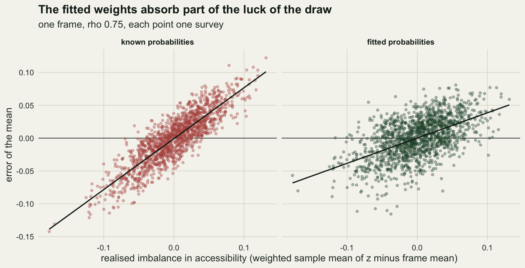
How much the fitted weights gain
The gain depends on how strongly accessibility predicts the response, and on the design. The main simulation runs the three values of rho on five fresh frames each, with 1500 surveys per frame. A second design with a lower intercept, plogis(-2 + z), visits far fewer sites and is run on three frames per rho, as a check on how much of the result belongs to the sample size. The headline ratio is the standard deviation of the fitted-weight mean over that of the known-weight mean, over repeated surveys of one fixed frame.
n_fr   <- c(5L, 3L)
a_set  <- c(a_int, -2)

summarise_frame <- function(fr, sims, rho, a0, k) {
  r12 <- cor(sims["m_e", ], sims["m_k", ])
  ratio <- sd(sims["m_e", ]) / sd(sims["m_k", ])
  cover <- function(m, v) mean(abs(sims[m, ] - fr$mu) <= z_crit * sqrt(sims[v, ]))
  data.frame(rho = rho, a0 = a0, frame = k, n_vis = mean(sims["n_vis", ]),
    bias_plain = mean(sims["plain", ]) - fr$mu,
    bias_k = mean(sims["m_k", ]) - fr$mu, bias_e = mean(sims["m_e", ]) - fr$mu,
    ratio = ratio, ratio_se = ratio * sqrt((1 - r12^2) / (ncol(sims) - 1)),
    cov_k = cover("m_k", "v_k"), cov_e = cover("m_e", "v_e"), cov_c = cover("m_e", "v_c"), cov_r = cover("m_e", "v_r"),
    neg_c = mean(sims["v_c", ] <= 0),
    cov_oracle = mean(abs(sims["m_e", ] - fr$mu) <= z_crit * sd(sims["m_e", ])),
    vr_k = mean(sims["v_k", ]) / var(sims["m_k", ]),
    vr_e = mean(sims["v_e", ]) / var(sims["m_e", ]),
    vr_c = mean(sims["v_c", ]) / var(sims["m_e", ]),
    cv_se_k = sd(sqrt(sims["v_k", ])) / mean(sqrt(sims["v_k", ])),
    cv_se_c = sd(sqrt(sims["v_c", ])) / mean(sqrt(sims["v_c", ])),
    cv_se_r = sd(sqrt(sims["v_r", ])) / mean(sqrt(sims["v_r", ])),
    sd_known = sd(sims["m_k", ]))
}

set.seed(4103)
frames <- list()
main_out <- do.call(rbind, lapply(seq_along(a_set), function(d) {
  do.call(rbind, lapply(rho_set, function(rho) {
    do.call(rbind, lapply(seq_len(n_fr[d]), function(k) {
      fr <- make_frame(rho, function(z) p_smooth(z, a_set[d]))
      frames[[length(frames) + 1]] <<- c(fr, rho = rho, a0 = a_set[d])
      sims <- replicate(n_rep, one_survey(fr, cbind(1, fr$z)))
      summarise_frame(fr, sims, rho, a_set[d], k)
    }))
  }))
}))

big  <- main_out[main_out$a0 == a_int, ]
small <- main_out[main_out$a0 != a_int, ]
by_rho <- function(tab, col, fun = mean) unname(tapply(tab[[col]], tab$rho, fun))
ratio_big  <- by_rho(big, "ratio");  ratio_small <- by_rho(small, "ratio")
ratio_lo   <- by_rho(big, "ratio", min); ratio_hi <- by_rho(big, "ratio", max)
ratio_se_max <- max(big$ratio_se)
bias_plain <- by_rho(big, "bias_plain")
bias_kmax  <- max(abs(main_out$bias_k)); bias_emax <- max(abs(main_out$bias_e))
sd_known_big <- by_rho(big, "sd_known")
nvis_big <- mean(big$n_vis); nvis_small <- mean(small$n_vis)
p_min_small <- min(vapply(frames[vapply(frames, function(f) f$a0 != a_int, TRUE)],
                          function(f) min(f$p), 0))
The plain mean of the visited sites is too high by 0.197, 0.370 and 0.463 at the three values of rho, which is what the weights are for. Both Hajek means are unbiased: across all 24 frames of both designs the largest bias is 0.0081 with the known probabilities and 0.0062 with the fitted ones.
In the main design, which visits 1247 sites on average, the standard deviation of the fitted-weight mean is 0.924, 0.801 and 0.704 times that of the known-weight mean at rho 0.40, 0.75 and 0.95 (means over five frames; the frame-to-frame range at rho 0.95 is 0.677 to 0.745, and the Monte Carlo standard error of any single frame’s ratio is at most 0.013). At the strongest link, estimating a probability that was never in doubt removes 30 per cent of the standard deviation of the mean. In the sparser design, visiting 463 sites, the ratios are 0.951, 0.880 and 0.823: still a gain, and a smaller one.
The R-squared rule gets the direction and not the size
A reader who knows the projection argument will predict the gain from the share of the response that accessibility explains: if a fraction rho squared of the variance is removable, the standard deviation ratio should be the square root of one minus rho squared. The exact projection says something narrower. The known-weight error is a sum of the centred visit indicators, each multiplied by the site’s deviation from the frame mean divided by its probability; the score of the logistic fit is a sum of the same indicators multiplied by one and by z. What the fit removes is the part of the first set of multipliers that a straight line in z can reproduce, in a least squares fit weighted by the Bernoulli variance p(1 - p). That weighted R-squared is computable from the responses over the frame, with no simulation of the draw.
proj_ratio <- function(fr) {
  u_i <- (fr$y - fr$mu) / fr$p
  w_i <- fr$p * (1 - fr$p)
  fit <- lm.wfit(cbind(1, fr$z), u_i, w_i)
  sqrt(sum(w_i * fit$residuals^2) / sum(w_i * u_i^2))
}
main_out$proj <- vapply(frames, proj_ratio, 0)
main_out$rule <- sqrt(1 - main_out$rho^2)
big  <- main_out[main_out$a0 == a_int, ]
small <- main_out[main_out$a0 != a_int, ]
proj_big <- by_rho(big, "proj"); proj_small <- by_rho(small, "proj")
rule_rho <- sqrt(1 - rho_set^2)
proj_miss <- max(abs(main_out$ratio - main_out$proj))
over_by   <- (1 - rule_rho[3]) / (1 - ratio_big[3])
The rule predicts ratios of 0.917, 0.661 and 0.312. The measured ratios in the main design are 0.924, 0.801 and 0.704, so at rho 0.95 the rule promises a cut in standard deviation 2.3 times the one delivered. The weighted projection, computed frame by frame, predicts 0.924, 0.803 and 0.710 for the main design and 0.956, 0.865 and 0.826 for the sparse one, and across all 24 frames it sits within 0.027 of the simulated ratio.
The rule fails because the multiplier that matters is the deviation divided by the probability, not the deviation. Dividing by a logistic curve in z bends a straight-line response into something a straight line in z cannot follow, most of all at the inaccessible end where the probabilities are small and the multipliers large, and the sparser design makes those small probabilities smaller. The gain is a property of how the response relates to the weights, which is why the same rho buys less in the sparse design.
rule_df <- data.frame(rho = seq(0.3, 0.97, by = 0.01))
rule_df$rule <- sqrt(1 - rule_df$rho^2)
proj_df <- aggregate(proj ~ rho + a0, data = main_out, FUN = mean)
lab_design <- function(a0) ifelse(a0 == a_int, "about 1250 sites visited", "about 470 sites visited")
main_out$design <- lab_design(main_out$a0)
proj_df$design  <- lab_design(proj_df$a0)
ggplot(main_out, aes(rho, ratio, colour = design)) +
  geom_line(data = rule_df, aes(rho, rule), inherit.aes = FALSE,
            linetype = "dashed", colour = te_body, linewidth = 0.6) +
  geom_line(data = proj_df, aes(rho, proj, colour = design), linewidth = 0.8) +
  geom_point(position = position_jitter(width = 0.008, height = 0, seed = 1),
             size = 2.2, alpha = 0.8) +
  annotate("text", x = 0.60, y = 0.66, label = "R-squared rule", colour = te_body,
           hjust = 0, size = 3.6) +
  scale_colour_manual(values = c(te_forest, te_gold), name = NULL) +
  scale_x_continuous(breaks = rho_set) +
  labs(x = "rho, correlation of the response with accessibility",
       y = "sd with fitted weights / sd with known",
       title = "The gain is real and smaller than the rule",
       subtitle = "points: frames; lines: weighted projection; dashed: R-squared rule") +
  theme_datasheet() +
  theme(legend.position = "bottom")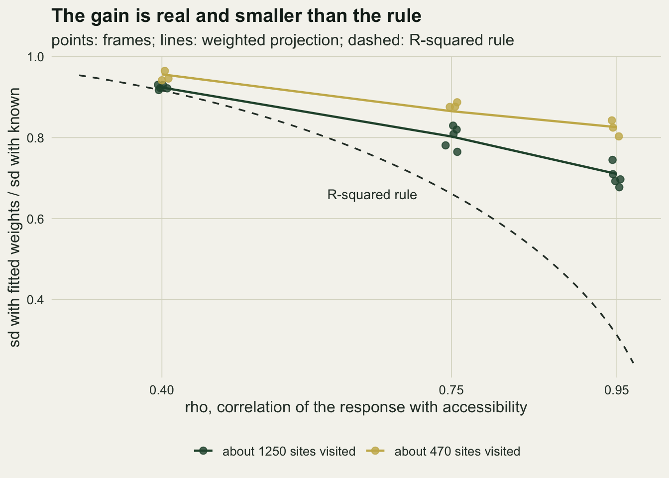
The textbook interval hands the gain back
The fitted-weight mean is more precise, but the variance formula a reader reaches for treats the probabilities as fixed and knows nothing about the fit. Paired with the fitted probabilities it estimates, near enough, the variance of the known-weight mean, which is larger. So the interval is too wide, and the precision gained in the estimate is lost again in what is reported about it.
mc_se_cov <- function(cv, n) sqrt(cv * (1 - cv) / n)
n_big   <- n_fr[1] * n_rep
cov_tab <- aggregate(cbind(cov_k, cov_e, cov_c, cov_r, cov_oracle, vr_k, vr_e, vr_c,
                           cv_se_k, cv_se_c, cv_se_r) ~ rho + a0, data = main_out, FUN = mean)
cb <- cov_tab[cov_tab$a0 == a_int, ]
cs <- cov_tab[cov_tab$a0 != a_int, ]
# standard error of a pooled coverage from the spread between frames
fr_se <- aggregate(cbind(cov_k, cov_e, cov_c) ~ rho + a0, data = main_out,
                   FUN = function(v) sd(v) / sqrt(length(v)))
fb <- fr_se[fr_se$a0 == a_int, ]
fs <- fr_se[fr_se$a0 != a_int, ]
se_fr_big <- range(c(fb$cov_k, fb$cov_c))
n_neg_c <- sum(main_out$neg_c * n_rep)
n_surv  <- nrow(main_out) * n_rep
short_c <- 0.95 - cb$cov_c; short_k <- 0.95 - cb$cov_k
short_z <- min(c(short_c[2:3] / fb$cov_c[2:3], short_k[2:3] / fb$cov_k[2:3]))
cc_95 <- big$cov_c[big$rho == 0.95]
se_cov_big <- mc_se_cov(0.95, n_big)
In the main design the textbook interval with the known probabilities covers the frame mean in 0.946, 0.933 and 0.937 of surveys at the three values of rho. The same formula around the fitted-weight mean covers in 0.966, 0.981 and 0.991: its average variance estimate is 1.18, 1.53 and 1.98 times the variance it is meant to estimate. With the corrected variance the coverage is 0.950, 0.932 and 0.926. Each coverage figure pools 7500 surveys, so its binomial Monte Carlo standard error near 0.95 is about 0.0025, but that treats five frames as one. Coverage also varies from frame to frame, and the standard error computed from the spread of the five frame-level coverages is 0.0030 to 0.0050 for the known-weight and corrected intervals, up to twice the binomial one.
This is the structural fact of the goodness-of-fit post in a different place. There the distance with estimated parameters was smaller than the table assumed, and the test built on the table almost never rejected. Here the spread of the mean with estimated probabilities is smaller than the formula assumes, and the interval built on the formula misses less often than it claims to.
The corrected interval under-covers at rho 0.75 and 0.95, by at least 4 frame-level standard errors, and so does the textbook interval with known probabilities: by a similar amount at rho 0.75 (shortfalls of 0.018 and 0.017 below 0.95) and about half as much at 0.95 (0.013 against 0.024). At rho 0.95 the five frames give the corrected interval coverages from 0.911 to 0.938. The simulation can say where the shortfall comes from there. The corrected variance is right on average: its mean is 0.980 times the true variance. An interval built with the true standard deviation covers in 0.949, so the spread, not the shape, is what the interval gets wrong. What remains is noise in the variance estimate itself. Its square root varies from survey to survey with a coefficient of variation of 0.32, against 0.21 for the textbook standard error with known probabilities. The subtraction in v_corr is not the cause: the corrected variance was negative in none of the 36000 surveys, and v_resid, the same linearisation written as a sum of squared residuals that cannot go negative, covers in 0.924 at rho 0.95 with a coefficient of variation of 0.32. Both are sums of terms weighted by (1 - p)/p^2, so both lean on the few visited sites with small probabilities and large weights. An unstable standard error costs coverage the way a t interval with few degrees of freedom would, even when it is unbiased. The known-weight interval, whose standard error is steadier, shows a milder form of the same thing, at 0.937.
The sparse design makes it worse. Visiting about 463 sites, the corrected interval covers in 0.942, 0.918 and 0.901 (standard error from the spread between its three frames at most 0.0054), the textbook interval with known probabilities in 0.940, 0.926 and 0.916, and the textbook formula around the fitted-weight mean still over-covers at 0.953, 0.954 and 0.964. The smallest design probability in those frames is 0.0026, so the variance estimate leans on a few inaccessible sites with very large weights, and every linearised interval there is a large-sample device. The diagnosis is the same as before: at rho 0.95 an interval with the true standard deviation still covers in 0.954, while the corrected standard error has a coefficient of variation of 0.41, and the residual form covers in 0.898.
cov_long <- rbind(
  data.frame(cov_tab[, c("rho", "a0")], cover = cov_tab$cov_k,
             pair = "known probabilities, textbook variance"),
  data.frame(cov_tab[, c("rho", "a0")], cover = cov_tab$cov_e,
             pair = "fitted probabilities, textbook variance"),
  data.frame(cov_tab[, c("rho", "a0")], cover = cov_tab$cov_c,
             pair = "fitted probabilities, corrected variance"))
cov_long$pair <- factor(cov_long$pair, levels = unique(cov_long$pair))
cov_long$design <- factor(lab_design(cov_long$a0),
                          levels = c("about 1250 sites visited", "about 470 sites visited"))
n_mc <- ifelse(cov_long$a0 == a_int, n_fr[1], n_fr[2]) * n_rep
cov_long$half <- 2 * pmax(c(fr_se$cov_k, fr_se$cov_e, fr_se$cov_c),
                          mc_se_cov(cov_long$cover, n_mc))
ggplot(cov_long, aes(factor(rho), cover, colour = pair)) +
  geom_hline(yintercept = 0.95, linetype = "dashed", colour = te_body, linewidth = 0.5) +
  geom_errorbar(aes(ymin = cover - half, ymax = cover + half),
                position = position_dodge(width = 0.55), width = 0.25, linewidth = 0.5) +
  geom_point(position = position_dodge(width = 0.55), size = 2.4) +
  facet_wrap(~ design) +
  scale_colour_manual(values = c(te_ink, te_rust, te_forest), name = NULL) +
  labs(x = "rho", y = "coverage of the frame mean",
       title = "Keep the fitted weights, change the variance",
       subtitle = "dashed: nominal 0.95") +
  guides(colour = guide_legend(ncol = 1)) +
  theme_datasheet() +
  theme(legend.position = "bottom",
        strip.text = element_text(colour = te_ink, face = "bold"))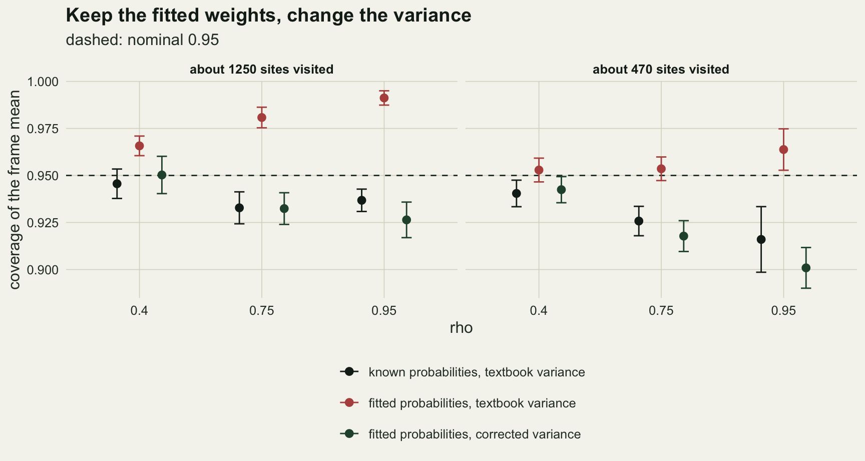
When the refitted model is wrong
Everything above refits the model that generated the design, so the fitted probabilities are consistent. A design is often simpler than a logistic curve. Suppose the coordinator put the sites into three accessibility bands, cutting z at -0.5 and 0.5, and gave them probabilities 0.15, 0.35 and 0.80. An analyst who refits a logistic regression in z now fits the wrong shape. Two refits cannot go wrong in that way: one fits a separate probability to each band, and the other keeps the known probability as an offset in the logistic regression and estimates an intercept and a slope in z on top of it, whose true values are both zero. The comparison runs at rho 0.75, on three frames with 1500 surveys each.
band_cut <- c(-Inf, -0.5, 0.5, Inf)
band_p   <- c(0.15, 0.35, 0.80)
p_band   <- function(z) band_p[findInterval(z, band_cut)]

band_survey <- function(fr, x_lin, x_band, off) {
  inc <- rbinom(n_site, 1L, fr$p); s <- which(inc == 1L); ys <- fr$y[s]
  p_lin <- logit_fit(inc, x_lin)
  p_bnd <- logit_fit(inc, x_band)
  p_off <- logit_fit(inc, x_lin, off = off)
  c(m_k = hajek(ys, fr$p[s]), m_lin = hajek(ys, p_lin[s]),
    m_bnd = hajek(ys, p_bnd[s]), m_off = hajek(ys, p_off[s]),
    v_k = v_text(ys, fr$p[s]),
    v_lin = v_corr(ys, p_lin[s], p_lin, x_lin, s),
    v_bnd = v_corr(ys, p_bnd[s], p_bnd, x_band, s),
    v_off = v_corr(ys, p_off[s], p_off, x_lin, s))
}

n_fr_band <- 3L
set.seed(4104)
band_raw <- list()
band_out <- do.call(rbind, lapply(seq_len(n_fr_band), function(k) {
  fr <- make_frame(0.75, p_band)
  band_f <- factor(findInterval(fr$z, band_cut))
  sims <- replicate(n_rep, band_survey(fr, cbind(1, fr$z),
                                       model.matrix(~ band_f), qlogis(fr$p)))
  est <- c("m_k", "m_lin", "m_bnd", "m_off"); vv <- c("v_k", "v_lin", "v_bnd", "v_off")
  band_raw[[k]] <<- data.frame(frame = k, err = as.vector(t(sims[est, ] - fr$mu)),
                               est = rep(est, each = n_rep))
  r_se <- function(e1) {
    r12 <- cor(sims[e1, ], sims["m_k", ])
    sqrt((1 - r12^2) / (n_rep - 1)) * sd(sims[e1, ]) / sd(sims["m_k", ])
  }
  data.frame(frame = k, est = est,
             ratio_se = c(0, r_se("m_lin"), r_se("m_bnd"), r_se("m_off")),
             bias = rowMeans(sims[est, ]) - fr$mu,
             sd = apply(sims[est, ], 1, sd),
             cover = vapply(seq_along(est), function(j)
               mean(abs(sims[est[j], ] - fr$mu) <= z_crit * sqrt(sims[vv[j], ])), 0))
}))
band_mean <- aggregate(cbind(bias, sd, cover) ~ est, data = band_out, FUN = mean)
bm <- function(e, col) band_mean[[col]][band_mean$est == e]
ratio_bnd <- bm("m_bnd", "sd") / bm("m_k", "sd")
ratio_off <- bm("m_off", "sd") / bm("m_k", "sd")
bias_in_sd <- abs(bm("m_lin", "bias")) / bm("m_k", "sd")
ratio_gap <- abs(ratio_bnd - ratio_off)
ratio_se_band <- max(band_out$ratio_se[band_out$est %in% c("m_bnd", "m_off")]) / sqrt(n_fr_band)
The logistic refit in z is biased by -0.167, which is 5.4 times the standard deviation of the known-weight mean, and its corrected interval covers in only 0.095 of surveys. The gain is gone and the unbiasedness with it: the fitted probabilities are no longer the design’s. The two refits that nest the design stay unbiased (bias -0.0004 with a probability per band and -0.0001 with the offset), and both still gain: their standard deviations are 0.708 and 0.721 times that of the known-weight mean, with corrected coverage of 0.948 and 0.948. The known-weight mean with the textbook variance covers in 0.948.
The per-band refit came out slightly ahead, by 0.013 in the ratio against a Monte Carlo standard error of up to 0.008 for each ratio averaged over the three frames; it fits one more free parameter than the offset refit. It is available only because this design has bands. The offset refit works for any design probability, smooth or stepped, and it cannot be misspecified in the direction that matters, because the design is the model with both extra coefficients at zero. With glm() it is one line, glm(visited ~ z, offset = qlogis(p_design), family = binomial), and further terms in z, or other frame variables, can be added to it without breaking that nesting.
band_all <- do.call(rbind, band_raw)
est_lab <- c(m_k = "known probabilities", m_lin = "logistic refit in z (wrong shape)",
             m_bnd = "refit, one probability per band", m_off = "logistic refit on the known offset")
band_all$label <- factor(est_lab[band_all$est], levels = rev(est_lab))
ggplot(band_all, aes(err, label)) +
  geom_vline(xintercept = 0, colour = te_body, linewidth = 0.5) +
  geom_boxplot(aes(fill = label), colour = te_ink, width = 0.55, outlier.size = 0.6,
               outlier.alpha = 0.4, linewidth = 0.4) +
  scale_fill_manual(values = c(te_forest, te_gold, te_rust, te_line), guide = "none") +
  labs(x = "error of the mean (estimate minus frame mean)", y = NULL,
       title = "A refit that nests the design keeps the gain",
       subtitle = paste0("rho 0.75; three frames, ", n_rep, " surveys each")) +
  theme_datasheet()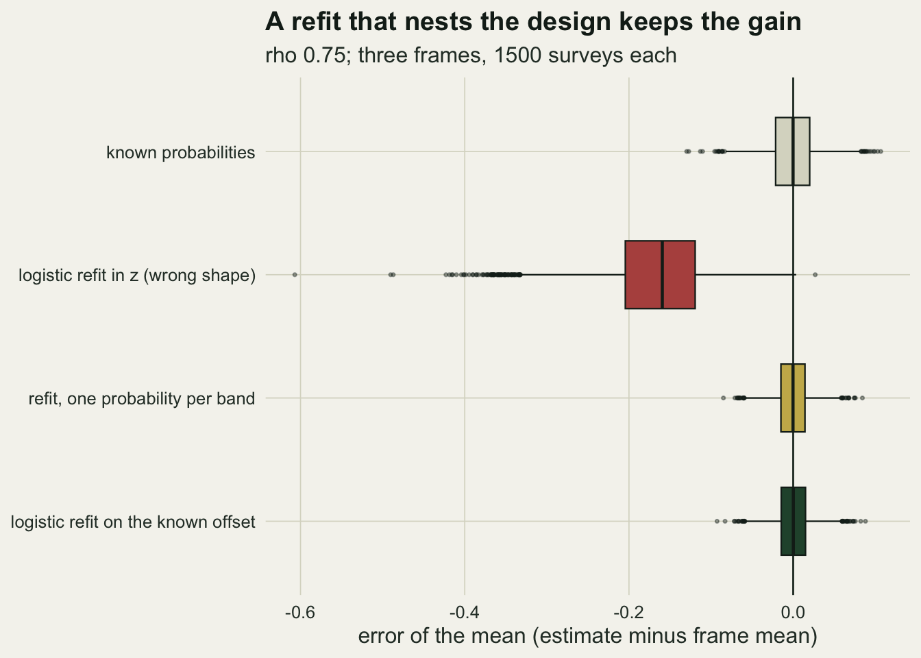
What to report
Say where the inclusion probabilities came from. If they were fixed by a draw the analyst made (Poisson sampling from a frame, another unequal-probability draw, a randomised follow-up of non-respondents at a fixed fraction as in Harvest surveys and the late respondent provided everyone subsampled is reached, or the second phase of a two-phase design), they are known exactly, and the question in this post applies, though only Poisson sampling was run here. If they were estimated because nothing else was available, as for non-response, there is no known value to compare against.
With known probabilities, report the Hajek mean with refitted probabilities, fitted on the known probability as an offset so that the refit nests the design, and say which variables the refit used. In the main design here, where a plain logistic refit already nests the design, refitting cut the standard deviation of the mean by 20 per cent at rho 0.75 and by 30 per cent at rho 0.95, for no bias. Do not predict the gain from the R-squared of the response on the design variable; the weighted projection (proj_ratio() in the section on the R-squared rule) predicts it from responses over the whole frame, which in practice means a pilot or a previous season’s data, and it matched the simulation to within 0.027 here.
Give the interval from the corrected variance, not from the textbook formula, and say which. The textbook formula around the fitted-weight mean covered in up to 0.991 of surveys in the main design, and the corrected one in 0.926 to 0.950. When the frame is small, the probabilities are small or the design variable predicts the response closely, say that the corrected interval is a large-sample interval, and that it under-covered at 0.901 in the sparse design here.
Honest limits
The design is Poisson sampling, where every site enters independently and the sample size is random. Most ecological designs fix the sample size: stratified random sampling, systematic grids, GRTS. There the analogue of refitting the probabilities is calibration or post-stratification on the design variable, which is related but is not the estimator run here, and its variance correction is different. Nothing above was run on a fixed-size design.
The response is linear in accessibility with normal noise. A response that is flat over most of the range and rises sharply near the tracks would change the weighted R-squared and so the gain; the projection chunk would still predict it, but the numbers here would not carry over.
The corrected variance is a linearisation. Its under-coverage at rho 0.95 and in the sparse design was traced to the instability of the variance estimate rather than to its bias, but no alternative was tried: neither a jackknife over the visited sites nor a bootstrap that redraws the Poisson sample and refits the probabilities each time. A reader with a small frame should try one of those and check it by simulation on their own frame before trusting either.
The misspecified arm has one wrong shape, a step design fitted with a smooth curve, at one value of rho. The size of the bias depends entirely on how wrong the refit is, and a refit that is only slightly wrong could still gain on balance. The safe advice, to refit on the known offset, does not depend on that.
Every frame here is a draw from a model with a known correlation, so the frame mean is known and the coverage can be scored. A real frame has one fixed set of responses. The projection chunk needs the responses over the whole frame and so cannot be run on real data before the survey; with a pilot or a previous season’s data it gives the expected gain for a planned design.
References
Henmi M, Eguchi S 2004 Biometrika 91(4):929-941 (10.1093/biomet/91.4.929)
Rosenbaum PR 1987 Journal of the American Statistical Association 82(398):387-394 (10.1080/01621459.1987.10478441)
Hirano K, Imbens GW, Ridder G 2003 Econometrica 71(4):1161-1189 (10.1111/1468-0262.00442)
Kim JK, Kim JJ 2007 Canadian Journal of Statistics 35(4):501-514 (10.1002/cjs.5550350403)