library(ggplot2)
library(patchwork)

te_paper  <- "#f5f4ee"
te_ink    <- "#16241d"
te_body   <- "#2c3a31"
te_forest <- "#275139"
te_rust   <- "#b5534e"
te_gold   <- "#c9b458"
te_line   <- "#dad9ca"

theme_datasheet <- function() {
  theme_minimal(base_size = 12) +
    theme(plot.background  = element_rect(fill = te_paper, colour = NA),
          panel.background = element_rect(fill = te_paper, colour = NA),
          panel.grid.major = element_line(colour = te_line, linewidth = 0.3),
          panel.grid.minor = element_blank(),
          text             = element_text(colour = te_body),
          plot.title       = element_text(colour = te_ink, face = "bold"),
          plot.subtitle    = element_text(colour = te_body),
          axis.text        = element_text(colour = te_body))
}

alpha_nom <- 0.05; n_obs <- 50L
mu_true   <- 64;   sd_true <- 2.1

set.seed(614)
wing   <- rnorm(n_obs, mu_true, sd_true)
mu_hat <- mean(wing)
sd_hat <- sd(wing)

ks_mle   <- suppressWarnings(ks.test(wing, "pnorm", mu_hat, sd_hat))
ks_truth <- ks.test(wing, "pnorm", mu_true, sd_true)
d_one_mle <- unname(ks_mle$statistic);   p_one_mle <- ks_mle$p.value
d_one_tab <- unname(ks_truth$statistic); p_one_tab <- ks_truth$p.valueTesting a fitted distribution
R
goodness of fit
model checking
resampling
ecology tutorial
Kolmogorov-Smirnov and Anderson-Darling go badly conservative once parameters are estimated. Measure the damage in R and repair it with a parametric bootstrap.
A ringing team measures wing chord on a season of adult reed warblers and wants a normal distribution for the trap: a normal prediction interval to flag birds worth a second look, a normal-theory interval on the seasonal mean. Before any of that, somebody checks. The check is one line, ks.test(x, "pnorm", mean(x), sd(x)), it returns a large p-value, and the sentence that goes into the report is that the data are consistent with a normal distribution.
That sentence is close to empty. The critical values Massey tabulated for the Kolmogorov-Smirnov distance, and the ones Anderson and Darling derived for their statistic, describe how far an empirical distribution function strays from a curve fixed before the data arrived. Estimating the mean and the standard deviation from the same sample moves the curve towards the data, the distance shrinks, and the test compares that shrunken distance against a table built for the unshrunken one. The test becomes conservative: it passes almost everything.
This post measures how conservative, at one sample size, with the replication fixed in advance, and then measures what the calibration is worth. The site already builds parametric bootstrap goodness-of-fit nulls in five places: the N-mixture check, the detection covariate post for spatial capture-recapture, the dynamic occupancy check, the multi-state check and the integrated SDM check. Only one of them, the dynamic occupancy check, names estimated parameters as the reason the reference distribution cannot be borrowed; the N-mixture check blames the mixture instead, and the other three build a statistic by hand that never had a table to lose. None of the five measures what the shortcut would have cost. The machinery is already written up in the parametric bootstrap post, where the asymptotic null fails because the null value sits on a boundary; here it fails because the curve was fitted to the same data, and what is new is the size and the power, measured.
The gap has a live consequence on this site. The GLM residual diagnostics post runs ks.test against a uniform on simulation-based quantile residuals from a fitted negative binomial, and reads the resulting large p-value as evidence that the model fits. Those residuals come from a model whose coefficients and dispersion were estimated from the same counts, so the uniform reference behind that p-value is not the right one, and the bias runs in the direction that flatters the model. That post does not say so. This one does, and the closing sections say what the honest version of the sentence looks like.
The same sample gives two different p-values
One season of ringing, wing chord in mm, and a known truth so the test can be scored.
The data really are normal, so both calls test a true hypothesis. Plugging the estimates in gives a distance of 0.0707 and a p-value of 0.949. Using the parameters the birds were generated from gives a distance of 0.1262 and a p-value of 0.372. Same birds, same test, and the plug-in version looks far more comfortable, because the fitted curve has been pulled towards the sample.
Two statistics are needed below, on many samples at a time, so they are written as functions over the columns of a matrix. The Kolmogorov-Smirnov distance is the largest vertical gap between the empirical distribution function and the fitted one. The Anderson-Darling statistic, from the asymptotic theory Anderson and Darling published in 1952 and the test they set out in 1954, is a weighted integral of the squared gap, with the weight rising in both tails. A hand-written statistic is a hypothesis until it is checked, so two checks follow the definitions: ks_dist must reproduce what ks.test reports, and both statistics must be unchanged when the sample is shifted and rescaled, since that invariance is what makes a single table possible at all.
sort_cols <- function(mat) {           # sort every column, without apply()
  n <- nrow(mat); m <- ncol(mat)
  matrix(mat[order(rep.int(seq_len(m), rep.int(n, m)), mat)], n, m)
}
col_max <- function(mat)
  mat[cbind(max.col(t(mat), ties.method = "first"), seq_len(ncol(mat)))]

zed <- function(mat, use_mle = TRUE, mu = 0, sdv = 1) {
  n <- nrow(mat)
  if (use_mle) {
    mu  <- colMeans(mat)
    sdv <- sqrt(colSums((mat - rep(mu, each = n))^2) / (n - 1))
  }
  sort_cols((mat - rep(mu, each = n)) / rep(sdv, each = n))
}

ks_dist <- function(mat, use_mle = TRUE, mu = 0, sdv = 1) {
  n  <- nrow(mat)
  fz <- pnorm(zed(mat, use_mle, mu, sdv))
  ii <- seq_len(n)
  pmax(col_max(ii / n - fz), col_max(fz - (ii - 1) / n))
}

ad_stat <- function(mat, use_mle = TRUE, mu = 0, sdv = 1) {
  n  <- nrow(mat)
  fz <- pmin(pmax(pnorm(zed(mat, use_mle, mu, sdv)), 1e-12), 1 - 1e-12)
  ii <- seq_len(n)
  -n - colSums((2 * ii - 1) * (log(fz) + log(1 - fz[n:1, , drop = FALSE]))) / n
}

set.seed(77)
chk_mat  <- matrix(rnorm(n_obs * 200, mu_true, sd_true), n_obs, 200)
gap_stat <- max(abs(ks_dist(chk_mat) -
  apply(chk_mat, 2, function(x)
    suppressWarnings(ks.test(x, "pnorm", mean(x), sd(x))$statistic))))
gap_scale <- max(abs(ks_dist(chk_mat * 7.3 - 40) - ks_dist(chk_mat)))
The largest disagreement with ks.test over two hundred samples is 6.3e-15, and the largest change under a shift and a rescale is 8.6e-15. Both are floating point noise, so the implementation is the same statistic and it is invariant to location and scale.
x_grid <- seq(min(wing) - 2, max(wing) + 2, length.out = 400)
cdf_long <- data.frame(x = rep(x_grid, 2),
  p = c(pnorm(x_grid, mu_hat, sd_hat), pnorm(x_grid, mu_true, sd_true)),
  which_curve = rep(c("parameters estimated from these birds",
                      "parameters fixed in advance"), each = length(x_grid)))

ggplot() +
  stat_ecdf(data = data.frame(x = wing), aes(x), geom = "step",
            colour = te_ink, linewidth = 0.7) +
  geom_line(data = cdf_long, aes(x, p, colour = which_curve), linewidth = 0.9) +
  scale_colour_manual(values = c(te_forest, te_rust), name = NULL) +
  labs(x = "wing chord (mm)", y = "cumulative probability",
       title = "The fitted curve is pulled towards the sample",
       subtitle = sprintf("largest gap: %.4f fitted, %.4f fixed",
                          d_one_mle, d_one_tab)) +
  theme_datasheet() +
  theme(legend.position = "bottom")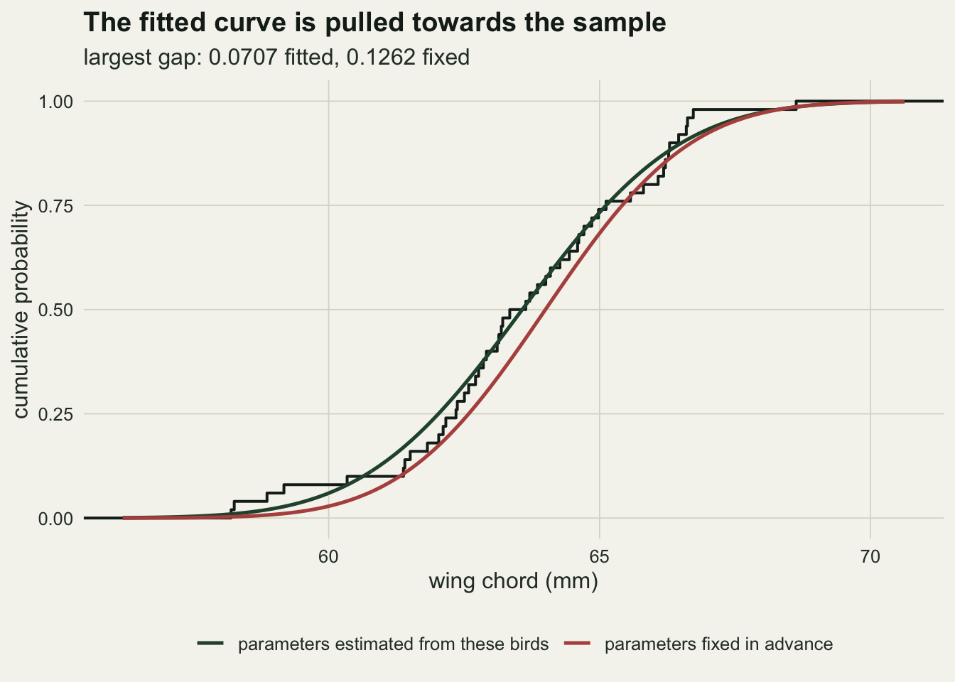
The null distribution is in the wrong place
The distance is smaller when the parameters are estimated, so its null distribution is shifted left and a table built for fixed parameters has its five per cent point too far to the right. Durbin set out why in general: once the parameters are estimated the empirical process is no longer a Brownian bridge, and the limiting covariance depends on the family and on the estimator, so there is no single table to borrow. Both nulls can be simulated in one pass over the same samples, once treating the generating parameters as known and once re-estimating them from every sample.
n_ref <- 20000L
set.seed(2026)
ref_mat <- matrix(rnorm(n_obs * n_ref), n_obs, n_ref)

d_tab <- ks_dist(ref_mat, use_mle = FALSE)
a_tab <- ad_stat(ref_mat, use_mle = FALSE)
d_mle <- ks_dist(ref_mat)
a_mle <- ad_stat(ref_mat)

five_pc <- function(v) unname(quantile(v, 1 - alpha_nom))
crit_d_tab <- five_pc(d_tab); crit_a_tab <- five_pc(a_tab)
crit_d_mle <- five_pc(d_mle); crit_a_mle <- five_pc(a_mle)

lil_crit   <- 0.886 / sqrt(n_obs)                          # Lilliefors 1967, n > 30
ad_tab_pub <- 2.492                                        # Stephens 1974, case 0
ad_mle_pub <- 0.752 / (1 + 0.75 / n_obs + 2.25 / n_obs^2)  # Stephens 1974, case 3

shrink_d <- crit_d_tab / crit_d_mle; shrink_a <- crit_a_tab / crit_a_mle
pc_gap   <- function(a, b) 100 * abs(a - b) / b
err_lil  <- pc_gap(crit_d_mle, lil_crit)
err_stp  <- pc_gap(crit_a_mle, ad_mle_pub)
err_tab  <- pc_gap(crit_a_tab, ad_tab_pub)
The simulation and the published tables have to agree before any of this is worth reading, and they do. With fixed parameters the five per cent point of the distance is 0.1881, and the Anderson-Darling five per cent point is 2.5045 against the 2.492 tabulated by Stephens, a difference of 0.5 per cent. With the parameters estimated, the distance five per cent point falls to 0.1243, against the 0.1253 Lilliefors published for this sample size, a difference of 0.8 per cent, and the Anderson-Darling point falls to 0.7385 against the 0.7402 implied by Stephens’s modified statistic, a difference of 0.2 per cent. Table and simulation agree on every one of them.
The size of the shift is the whole story. The tabulated critical distance is 1.51 times the one the plug-in statistic actually needs, and for Anderson-Darling the factor is 3.39. Anderson-Darling weights the tails, which is where estimating a standard deviation does most of its flattering, so it suffers more.
A parametric bootstrap reproduces the second null without a table. Simulate new samples from the fitted distribution, re-estimate the parameters on each one, recompute the statistic, and read the observed value against the spread of those values.
n_wingboot <- 20000L
set.seed(29)
wing_b  <- matrix(rnorm(n_obs * n_wingboot, mu_hat, sd_hat), n_obs, n_wingboot)
d_wing  <- ks_dist(wing_b)
a_wing  <- ad_stat(wing_b)
crit_d_wing <- five_pc(d_wing); crit_a_wing <- five_pc(a_wing)
p_wing_ks   <- (1 + sum(d_wing >= d_one_mle)) / (n_wingboot + 1)
p_wing_ad   <- (1 + sum(a_wing >= ad_stat(matrix(wing, ncol = 1)))) / (n_wingboot + 1)
The bootstrap five per cent points from this one sample of birds are 0.1247 and 0.7357, against 0.1243 and 0.7385 from the simulation that knew the truth. The bootstrap does not need the truth to land in the same place. Its p-value for these birds is 0.765 for the distance and 0.305 for Anderson-Darling, against the 0.949 that ks.test reported.
null_df <- function(from_table, from_boot) data.frame(
  stat = c(from_table, from_boot),
  which_null = rep(c("null the table assumes", "parametric bootstrap null"),
                   c(length(from_table), length(from_boot))))

null_panel <- function(dat, hi_line, lo_line, x_hi, x_lab, panel_title) {
  ggplot(dat, aes(stat, fill = which_null)) +
    geom_density(alpha = 0.55, colour = NA) +
    geom_vline(xintercept = c(lo_line, hi_line), colour = c(te_forest, te_gold),
               linetype = "dashed", linewidth = 0.7) +
    scale_fill_manual(values = c(te_gold, te_forest), name = NULL) +
    coord_cartesian(xlim = c(0, x_hi)) +
    labs(x = x_lab, y = "density", title = panel_title) +
    theme_datasheet()
}

p_left  <- null_panel(null_df(d_tab, d_wing), crit_d_tab, crit_d_wing, 0.32,
                      "Kolmogorov-Smirnov distance", "Distance")
p_right <- null_panel(null_df(a_tab, a_wing), crit_a_tab, crit_a_wing, 4,
                      "Anderson-Darling statistic", "Anderson-Darling")

(p_left + p_right) +
  plot_layout(guides = "collect") +
  plot_annotation(theme = theme_datasheet()) &
  theme(legend.position = "bottom")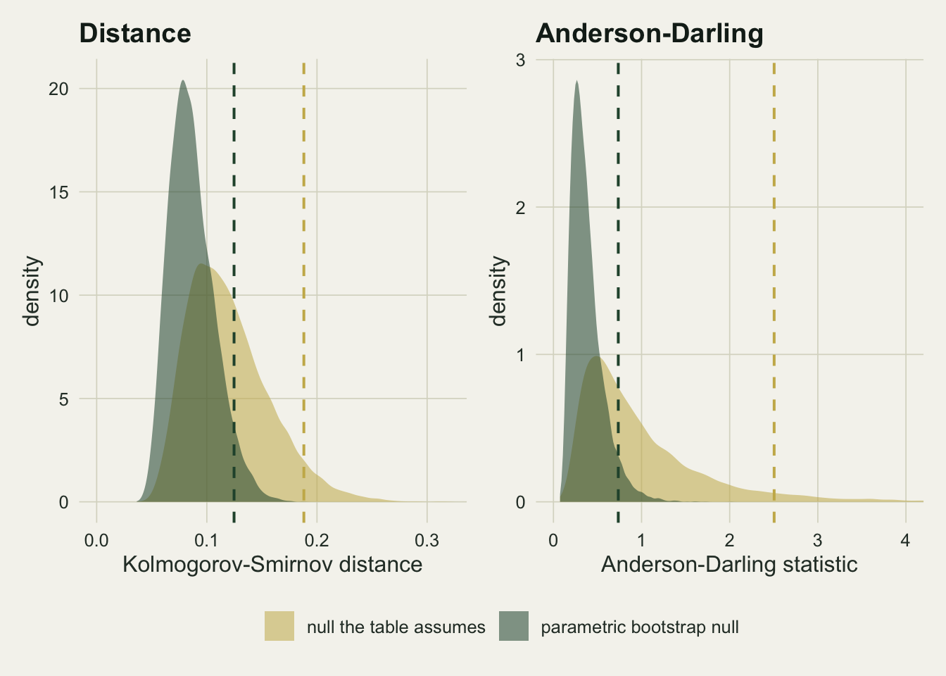
The test almost never rejects
A critical value in the wrong place is an abstraction; the rejection rate is not. That rate is a rare event here, so the replication has to be set by what the claim needs rather than by habit. The claim is that the true size is at least two orders of magnitude below the nominal one, which means resolving a rate near one in ten thousand, so the plug-in run uses a hundred thousand samples. The control with fixed parameters is a rate near one in twenty and needs far less, so it uses twenty thousand.
n_size <- 100000L
set.seed(11)
p_naive <- replicate(n_size, {
  x <- rnorm(n_obs, mu_true, sd_true)
  suppressWarnings(ks.test(x, "pnorm", mean(x), sd(x))$p.value)
})
size_naive <- mean(p_naive < alpha_nom)
mcse_naive <- sqrt(size_naive * (1 - size_naive) / n_size)
hits_naive <- round(size_naive * n_size)
hi_naive   <- qgamma(1 - alpha_nom / 2, hits_naive + 1) / n_size
lo_naive   <- qgamma(alpha_nom / 2, hits_naive) / n_size
ratio_low  <- alpha_nom / hi_naive; one_in <- 1 / hi_naive
span_naive <- hi_naive / lo_naive

n_ctrl <- 20000L
set.seed(12)
p_ctrl <- replicate(n_ctrl,
  ks.test(rnorm(n_obs, mu_true, sd_true), "pnorm", mu_true, sd_true)$p.value)
size_ctrl <- mean(p_ctrl < alpha_nom)
mcse_ctrl <- sqrt(size_ctrl * (1 - size_ctrl) / n_ctrl)

n_big <- 100000L                       # Anderson-Darling, vectorised
set.seed(13)
hits_ad <- 0L; hits_ks <- 0L
for (blk in 1:5) {
  blk_mat <- matrix(rnorm(n_obs * 20000L, mu_true, sd_true), n_obs, 20000L)
  hits_ad <- hits_ad + sum(ad_stat(blk_mat) > crit_a_tab)
  hits_ks <- hits_ks + sum(ks_dist(blk_mat) > crit_d_tab)
}
size_ad_naive <- hits_ad / n_big
size_ks_vec   <- hits_ks / n_big
rule_three    <- 3 / n_big
With the parameters fixed in advance, ks.test rejects a true normal hypothesis in 0.0478 of samples, with a Monte Carlo standard error of 0.0015. That is the nominal rate, and it says the machinery is sound: the statistic, the exact null and the tail probability are all correct. Nothing is broken in ks.test.
Swap mean(x) and sd(x) in for those parameters and the rejection rate collapses to 0.00013, with a Monte Carlo standard error of 0.00004. The count behind that rate is small, so the rate itself is loosely determined and the honest statement is the bound: the upper limit of the interval is 0.00022, which puts the nominal level at least 225 times above the size the test actually has. A test advertised to reject one true hypothesis in twenty rejects fewer than one in 4498.
Anderson-Darling is worse, and its rejection rate is too rare to count with ks.test in a sensible time, so the vectorised statistic does the same run in blocks. The vectorised distance gives 0.00016, agreeing with ks.test on an independent set of samples. Anderson-Darling with plug-in estimates crossed its simulated five per cent point in 0 of 100,000 samples, so the only defensible statement is the rule of three: its size is below 0.00003. Passing that test is not evidence of anything.
A parametric bootstrap puts the size back
The repair is to stop borrowing a table and build the null from the fitted model, the recipe the site already uses for hierarchical models and the one Stute, Gonzalez Manteiga and Presedo Quindimil justified for this class of statistic. Simulate from the fit, re-estimate on every simulated dataset, and read the observed statistic against those draws.
n_boot <- 999L; n_cal <- 2000L

boot_gof <- function(x, n_sim = n_boot) {
  x_mat <- matrix(x, ncol = 1)
  sim   <- matrix(rnorm(length(x) * n_sim, mean(x), sd(x)), length(x), n_sim)
  d_sim <- ks_dist(sim)
  a_sim <- ad_stat(sim)
  c(ks   = (1 + sum(d_sim >= ks_dist(x_mat))) / (n_sim + 1),
    ad   = (1 + sum(a_sim >= ad_stat(x_mat))) / (n_sim + 1),
    crit = unname(quantile(d_sim, 1 - alpha_nom)))
}

set.seed(31)
cal_out <- replicate(n_cal, boot_gof(rnorm(n_obs, mu_true, sd_true)))
size_boot_ks <- mean(cal_out["ks", ] < alpha_nom)
size_boot_ad <- mean(cal_out["ad", ] < alpha_nom)
mcse_boot    <- sqrt(alpha_nom * (1 - alpha_nom) / n_cal)

set.seed(33)
crit_spread <- sd(cal_out["crit", ])
mc_spread   <- sd(replicate(400,
  quantile(sample(d_mle, n_boot, replace = TRUE), 1 - alpha_nom)))
The calibrated size is 0.0540 for the distance and 0.0540 for Anderson-Darling, against a nominal 0.05 with a Monte Carlo standard error of 0.0049. Both are within one standard error of the level they advertise. The bootstrap costs 999 extra simulated samples per dataset and it buys a test that means what it says.
One measurement explains why so few bootstrap replicates are needed. Across the 2000 calibration datasets the bootstrap five per cent point varied with a standard deviation of 0.00197, while resampling the same number of draws from a single fixed null gives a standard deviation of 0.00194. The two agree, so the per-dataset nulls differ only by Monte Carlo noise, not by the estimates they were built from. For a location and scale family this is exact: the statistic is invariant to shift and rescale, as the check in the first section showed, so the null cannot depend on where the fitted curve sits. That is why Lilliefors could publish a table at all, and it is why the power study below can use one pooled null instead of rebuilding it for every dataset.
size_dat <- data.frame(
  setting = c("fixed parameters, table", "estimated, KS table", "estimated, AD table",
              "estimated, KS bootstrap", "estimated, AD bootstrap"),
  rate = c(size_ctrl, size_naive, size_ad_naive, size_boot_ks, size_boot_ad),
  reps = c(n_ctrl, n_size, n_big, n_cal, n_cal),
  kind = c("fixed", "table", "table", "bootstrap", "bootstrap"))
size_dat$setting <- factor(size_dat$setting, levels = rev(size_dat$setting))
size_dat$hits <- round(size_dat$rate * size_dat$reps)
is_bound <- size_dat$hits == 0                 # rule of three when nothing rejected
size_dat$lo <- qgamma(alpha_nom / 2, size_dat$hits) / size_dat$reps
size_dat$hi <- ifelse(is_bound, 3 / size_dat$reps,
  qgamma(1 - alpha_nom / 2, size_dat$hits + 1) / size_dat$reps)
size_dat$shown  <- ifelse(is_bound, "bound", "measured")
size_dat$marker <- ifelse(is_bound, size_dat$hi, size_dat$rate)
size_dat$note   <- ifelse(is_bound, sprintf("no rejections in %s: at most %.5f",
  formatC(size_dat$reps, format = "d", big.mark = ","), size_dat$hi), "")

ggplot(size_dat, aes(marker, setting, colour = kind)) +
  geom_vline(xintercept = alpha_nom, colour = te_rust,
             linetype = "dashed", linewidth = 0.8) +
  geom_errorbar(aes(xmin = lo, xmax = hi), orientation = "y",
                width = 0.25, linewidth = 0.6) +
  geom_point(aes(shape = shown), size = 3, stroke = 1.1, fill = te_paper) +
  geom_text(aes(label = note), hjust = 0, nudge_x = 0.022, size = 3.2,
            colour = te_body) +
  scale_shape_manual(values = c(bound = 21, measured = 16), guide = "none") +
  scale_colour_manual(values = c(te_forest, te_ink, te_gold), guide = "none") +
  scale_x_sqrt(breaks = c(0, 1e-3, 1e-2, 5e-2),
               labels = function(v) formatC(v, format = "fg", drop0trailing = TRUE),
               expand = expansion(mult = c(0.02, 0.08))) +
  labs(x = "rejection rate of a true hypothesis (square-root scale)", y = NULL,
       title = "The table only works when nothing was estimated",
       subtitle = "dashed red: nominal five per cent; bars are 95 per cent intervals") +
  theme_datasheet()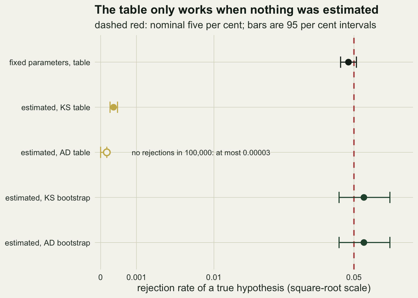
Calibration multiplies the power
A conservative test is not merely cautious, it is deaf, and the cost is measured against alternatives it ought to catch. The alternatives here are a Student t, whose tails are heavier than a normal’s by an amount the degrees of freedom control, and a contaminated normal in which a tenth of the birds come from a wider distribution. Four thousand replicates per setting were fixed in advance, which gives a Monte Carlo standard error of at most eight tenths of a percentage point: enough to separate rates that differ by tens of points, not enough to chase small ones.
n_pow <- 4000L; df_seq <- c(2, 3, 4, 6, 10, 20)

set.seed(41)
pow_tab <- t(sapply(df_seq, function(dfv) {
  alt   <- matrix(rt(n_obs * n_pow, dfv), n_obs, n_pow)
  d_alt <- ks_dist(alt)
  a_alt <- ad_stat(alt)
  c(ks_table = mean(d_alt > crit_d_tab), ks_boot = mean(d_alt > crit_d_mle),
    ad_table = mean(a_alt > crit_a_tab), ad_boot = mean(a_alt > crit_a_mle))
}))
rownames(pow_tab) <- df_seq
mcse_pow <- sqrt(0.25 / n_pow)

set.seed(45)
null_alt <- matrix(rnorm(n_obs * n_pow, mu_true, sd_true), n_obs, n_pow)
size_pooled_ks <- mean(ks_dist(null_alt) > crit_d_mle)
size_pooled_ad <- mean(ad_stat(null_alt) > crit_a_mle)

set.seed(47)
mix_frac <- 0.10; mix_sd <- 3
mix_alt  <- matrix(rnorm(n_obs * n_pow) *
  ifelse(runif(n_obs * n_pow) < mix_frac, mix_sd, 1), n_obs, n_pow)
mix_ks_table <- mean(ks_dist(mix_alt) > crit_d_tab)
mix_ks_boot  <- mean(ks_dist(mix_alt) > crit_d_mle)
mix_ad_table <- mean(ad_stat(mix_alt) > crit_a_tab)
mix_ad_boot  <- mean(ad_stat(mix_alt) > crit_a_mle)

row_t3  <- pow_tab[as.character(3), ]
gain_ks <- unname(row_t3["ks_boot"] / row_t3["ks_table"])
gain_ad <- unname(row_t3["ad_boot"] / row_t3["ad_table"])
gain_mix_ks <- mix_ks_boot / mix_ks_table; gain_mix_ad <- mix_ad_boot / mix_ad_table
On a fresh set of normal samples the pooled calibrated critical values reject in 0.0485 and 0.0508 of cases, so the reference is honest and the rates below are power rather than leakage. The Monte Carlo standard error on each of them is at most 0.0079.
Against a t with three degrees of freedom, the plug-in distance compared against its table rejects in 0.100 of samples and the calibrated version in 0.469, a factor of 4.7. For Anderson-Darling the pair is 0.107 and 0.591, a factor of 5.5. Against the contaminated normal the calibrated distance rejects in 0.310 of samples against 0.020 uncalibrated, a factor of 15.3, and calibrated Anderson-Darling reaches 0.457 against 0.031, a factor of 14.9. Calibration is not tidying up after the fact. It is most of the test.
The second pattern is that Anderson-Darling beats the distance once both are calibrated: 0.591 against 0.469 at three degrees of freedom, and 0.457 against 0.310 on the mixture. Both alternatives differ from a normal mainly in the tails, where the Anderson-Darling weight is largest, while the Kolmogorov-Smirnov distance is usually attained near the middle.
pow_long <- data.frame(
  df    = rep(df_seq, 4),
  power = as.vector(pow_tab),
  stat_id = rep(c("Kolmogorov-Smirnov", "Anderson-Darling"), each = 2 * length(df_seq)),
  null_id = rep(rep(c("tabulated null", "bootstrap null"), each = length(df_seq)), 2))

ggplot(pow_long, aes(df, power, colour = stat_id, linetype = null_id)) +
  geom_hline(yintercept = alpha_nom, colour = te_rust,
             linetype = "dashed", linewidth = 0.6) +
  geom_line(linewidth = 0.9) +
  geom_point(size = 2) +
  scale_x_log10(breaks = df_seq) +
  scale_colour_manual(values = c(te_gold, te_forest), name = NULL) +
  scale_linetype_manual(values = c("solid", "dotted"), name = NULL) +
  labs(x = "degrees of freedom of the t alternative", y = "rejection rate",
       title = "What the wrong null costs",
       subtitle = "dashed red: the nominal five per cent") +
  theme_datasheet() +
  theme(legend.position = "bottom")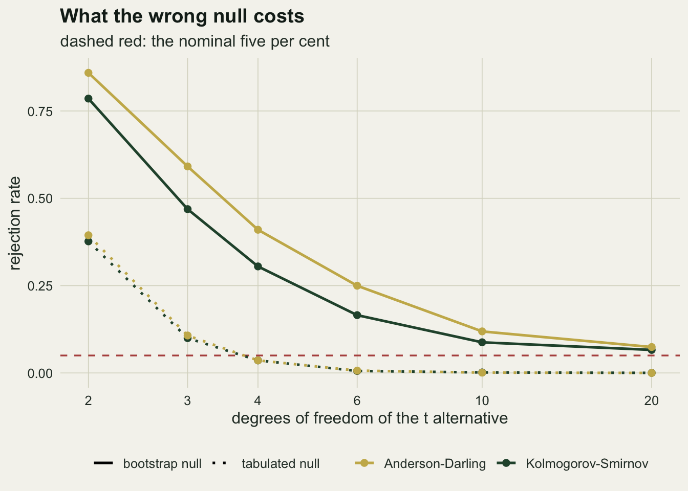
What to report
Say which parameters were estimated from the data being tested. That one sentence decides whether the p-value has a meaning, and it is the thing missing from most reported goodness-of-fit tests. If nothing was estimated, the table applies and ks.test is complete as it stands.
If anything was estimated, report the statistic and a bootstrap p-value, and give the number of simulated datasets that produced it. A bootstrap p-value from 999 draws cannot be smaller than one over that number plus one, so quote it as a bound when it hits the floor rather than writing zero.
Give the sample size with the result, and where a published table covers the exact case, use it and say so. For a normal with both parameters estimated, Lilliefors gives the distance and Stephens gives the modified Anderson-Darling, and both agreed with the bootstrap here to within one per cent. The bootstrap earns its keep when the fitted model is anything a table does not cover, which is the usual situation in ecology.
Report a failure to reject as what it is. “The Kolmogorov-Smirnov test did not reject normality” describes the analyst’s action, not the data, and when the parameters were plugged in it describes a test that rejects fewer than one true hypothesis in 4498.
Honest limits
Everything measured here is for one distribution at one sample size: a normal with both parameters estimated, from fifty observations. The direction of the bias is general, because it follows from the fitted curve being closer to the sample than the true curve is, but the size of it is not. A different family, a different estimator or a different sample size gives a different number, and the only way to know which is to run the bootstrap.
The claim about the GLM residual diagnostics post needs the same care. The uniformity test on simulation-based quantile residuals is biased for the same reason, since the coefficients and the dispersion came from the same counts, and the bias flatters the model. How large it is there is a separate measurement that this post did not make, and it depends on the number of parameters relative to the sample. The repair is the same shape: simulate from the fit, refit, and recompute, which is what the refitted option in DHARMa does and what costs the time.
The bootstrap here is the simple version, because the normal location and scale family is invariant enough that the null does not depend on the estimates. That was measured rather than assumed, but it stops being true for families where a shape parameter is estimated, a gamma or a Weibull for instance. There the null does move with the fit, one null per dataset is required, and the number of simulated datasets stops being a free choice.
The rare-event rates are the weakest numbers in the post. The plug-in size rests on 13 rejections in 100,000 samples, which pins it only to within a factor of 3.2 end to end, and the Anderson-Darling size is known only as an upper bound. Every statement above about those rates is written as a bound for that reason, and raising the replication to tighten them would change no conclusion, because the conclusions rest on the critical values, which are measured to three digits.
The alternatives are heavy tailed by construction, which is the case both statistics are built for. A skewed alternative, or one that differs from a normal in the middle rather than the tails, could reorder the two statistics, and the site’s wider point about residual plots applies here as well: a global distance is one number, and one number cannot say where a distribution went wrong.
References
Massey FJ 1951 Journal of the American Statistical Association 46(253):68-78 (10.1080/01621459.1951.10500769)
Anderson TW, Darling DA 1952 The Annals of Mathematical Statistics 23(2):193-212 (10.1214/aoms/1177729437)
Anderson TW, Darling DA 1954 Journal of the American Statistical Association 49(268):765-769 (10.1080/01621459.1954.10501232)
Lilliefors HW 1967 Journal of the American Statistical Association 62(318):399-402 (10.1080/01621459.1967.10482916)
Durbin J 1973 The Annals of Statistics 1(2) (10.1214/aos/1176342365)
Stephens MA 1974 Journal of the American Statistical Association 69(347):730-737 (10.1080/01621459.1974.10480196)
Stute W, Gonzalez Manteiga W, Presedo Quindimil M 1993 Metrika 40(1):243-256 (10.1007/BF02613687)