Least-cost paths and resistance surfaces

Compute cost distance and least-cost paths in base R with iterative sweeps, then measure how much the answer depends on the resistance values you chose.

A resistance surface says how costly it is to cross each cell of a landscape, and a least-cost path is the cheapest route between two points across it. The pair is the workhorse of corridor planning: give the model a source, a destination and a resistance map, and it returns a line on a map that looks authoritative.

The line is only as good as the resistance values, and those are almost always assigned by expert judgement or by a habitat model with no movement data behind it. This tutorial implements cost distance and path tracing from scratch in base R, then measures how much of the answer the resistance values decide.

Cost distance without a package

Cost distance is a shortest-path problem on a grid graph, and it does not need a priority queue if you are willing to sweep. Start with infinite distance everywhere except the source, then repeatedly relax every cell against its eight neighbours until nothing changes. Each sweep is eight shifted-matrix comparisons, which is fast in R, and the number of sweeps needed is roughly the diameter of the grid.

library(ggplot2)

te_pal <- list(forest = "#275139", green = "#2f8f63", sage = "#93a87f",
               clay = "#b5534e", gold = "#cda23f", line = "#dad9ca",
               ink = "#16241d", paper = "#f5f4ee")

theme_te <- function() {
  theme_minimal(base_size = 12) +
    theme(panel.grid.minor = element_blank(),
          panel.grid.major = element_line(colour = "#e7e6dc"),
          plot.background = element_rect(fill = "white", colour = NA),
          panel.background = element_rect(fill = "white", colour = NA),
          plot.title = element_text(face = "bold", colour = te_pal$ink),
          axis.title = element_text(colour = "#2c3a31"))
}

smooth_field <- function(n, passes, seed) {
  set.seed(seed)
  z <- matrix(runif(n * n), n, n)
  for (p in seq_len(passes)) {
    pad <- rbind(z[1, ], z, z[n, ])
    pad <- cbind(pad[, 1], pad, pad[, n])
    z <- (pad[1:n, 2:(n + 1)] + pad[3:(n + 2), 2:(n + 1)] +
            pad[2:(n + 1), 1:n] + pad[2:(n + 1), 3:(n + 2)] +
            4 * pad[2:(n + 1), 2:(n + 1)]) / 8
  }
  (z - min(z)) / (max(z) - min(z))
}

shift_mat <- function(m, dy, dx) {
  n <- nrow(m)
  p <- ncol(m)
  out <- matrix(Inf, n, p)
  yi <- max(1, 1 - dy):min(n, n - dy)
  xi <- max(1, 1 - dx):min(p, p - dx)
  out[yi, xi] <- m[yi + dy, xi + dx]
  out
}

cost_distance <- function(res, src, max_iter = 2000) {
  d <- matrix(Inf, nrow(res), ncol(res))
  d[src] <- 0
  moves <- list(c(-1, 0), c(1, 0), c(0, -1), c(0, 1),
                c(-1, -1), c(-1, 1), c(1, -1), c(1, 1))
  for (it in seq_len(max_iter)) {
    old <- d
    for (mv in moves) {
      step <- if (sum(abs(mv)) == 2) sqrt(2) else 1
      d <- pmin(d, shift_mat(d, mv[1], mv[2]) +
                  step * (res + shift_mat(res, mv[1], mv[2])) / 2)
    }
    if (max(abs(old - d)[is.finite(old) & is.finite(d)]) < 1e-9 &&
        sum(is.finite(d)) == sum(is.finite(old))) break
  }
  attr(d, "iterations") <- it
  d
}

trace_path <- function(d_from, start_idx) {
  n <- nrow(d_from)
  pos <- start_idx
  path <- pos
  moves <- expand.grid(dy = -1:1, dx = -1:1)
  moves <- moves[!(moves$dy == 0 & moves$dx == 0), ]
  repeat {
    yy <- ((pos - 1) %% n) + 1
    xx <- ((pos - 1) %/% n) + 1
    cand <- data.frame(y = yy + moves$dy, x = xx + moves$dx)
    cand <- cand[cand$y >= 1 & cand$y <= n &
                   cand$x >= 1 & cand$x <= ncol(d_from), ]
    vals <- d_from[cbind(cand$y, cand$x)]
    best <- which.min(vals)
    if (vals[best] >= d_from[pos]) break
    pos <- (cand$x[best] - 1) * n + cand$y[best]
    path <- c(path, pos)
    if (d_from[pos] == 0) break
  }
  path
}

The cost of stepping between two cells is the mean of their resistances times the step length, one for orthogonal moves and the square root of two for diagonals. That averaging convention matters: taking the destination cell’s resistance instead systematically undercounts the cost of leaving a cheap cell, and different software packages make different choices here.

Path tracing is the reverse operation. Once cost distance from the source is known everywhere, walking greedily downhill from the destination gives the least-cost path, because cost distance decreases monotonically along it.

One landscape, four resistance scales

The habitat quality surface is fixed. What varies is how much more expensive the worst cell is than the best, from a factor of five to a factor of a thousand: the same ranking of the landscape, four different contrasts.

n <- 100
quality <- smooth_field(n, 8, seed = 473)
src_a <- matrix(FALSE, n, n)
src_a[8, 8] <- TRUE
src_b <- matrix(FALSE, n, n)
src_b[93, 93] <- TRUE
idx_b <- (93 - 1) * n + 93
diag_cells <- cbind(round(seq(8, 93, length.out = 200)),
                    round(seq(8, 93, length.out = 200)))

contrast_run <- function(rmax) {
  res <- 1 + (rmax - 1) * (1 - quality)
  d_a <- cost_distance(res, src_a)
  d_b <- cost_distance(res, src_b)
  corridor <- d_a + d_b
  list(rmax = rmax, res = res, cost = d_a[idx_b],
       path = trace_path(d_a, idx_b), corridor = corridor,
       straight_cost = mean(res[diag_cells]) * sqrt(2) * 85,
       corridor_frac = mean(corridor <= 1.05 * min(corridor)),
       iters = attr(d_a, "iterations"))
}

runs <- lapply(c(5, 20, 100, 1000), contrast_run)
tab <- do.call(rbind, lapply(runs, function(r) data.frame(
  max_resistance = r$rmax, cost_distance = round(r$cost, 1),
  straight_line_cost = round(r$straight_cost, 1),
  detour_saving = round(1 - r$cost / r$straight_cost, 4),
  path_cells = length(r$path),
  corridor_share = round(r$corridor_frac, 4), sweeps = r$iters)))
print(tab, row.names = FALSE)

 max_resistance cost_distance straight_line_cost detour_saving path_cells
              5         388.4              404.4        0.0396         92
             20        1356.7             1470.1        0.0771        101
            100        6521.0             7153.9        0.0885        101
           1000       64619.8            71096.9        0.0911        101
 corridor_share sweeps
         0.3411    104
         0.3052    104
         0.3040    104
         0.3035    105

Three numbers in that table are worth reading carefully.

The detour saving is what the least-cost route buys over walking the straight line: 3.96 percent at a contrast of five, rising to 9.11 percent at a contrast of a thousand. On a smoothly varying surface there is simply not much to gain by going around, and the model’s own optimum is only slightly better than the naive route. That is not a defect of the method; it is information about the landscape, and it is worth computing before a corridor is drawn on the strength of the model.

The sweep count stays near 104 for a 100 by 100 grid, confirming that the iteration count follows the grid diameter rather than the resistance values.

The corridor share is the uncomfortable one. Adding cost distance from both endpoints gives, for every cell, the cost of the cheapest route through that cell, and cells within five percent of the global minimum form the usual definition of a corridor. That set covers 34.11 percent of the map at a contrast of five and about 30 percent at higher contrasts. The single least-cost line is one route through a very wide band of nearly equivalent routes, and drawing it as a line hides that.

r3 <- runs[[3]]
grid_df <- data.frame(
  x = rep(seq_len(n), each = n), y = rep(seq_len(n), times = n),
  resistance = as.vector(r3$res),
  in_corridor = as.vector(r3$corridor <= 1.05 * min(r3$corridor)))
path_df <- data.frame(y = ((r3$path - 1) %% n) + 1,
                      x = ((r3$path - 1) %/% n) + 1)

ggplot(grid_df, aes(x, y)) +
  geom_raster(aes(fill = resistance)) +
  geom_raster(data = subset(grid_df, in_corridor), fill = "white",
              alpha = 0.35) +
  geom_path(data = path_df, colour = te_pal$ink, linewidth = 0.8) +
  coord_equal() +
  scale_fill_gradient(low = te_pal$paper, high = te_pal$forest,
                      name = "resistance") +
  labs(title = "The corridor is wide, the path is one line through it",
       subtitle = "shaded: routes within five percent of the cheapest total cost",
       x = NULL, y = NULL) +
  theme_te() +
  theme(axis.text = element_blank(), panel.grid = element_blank())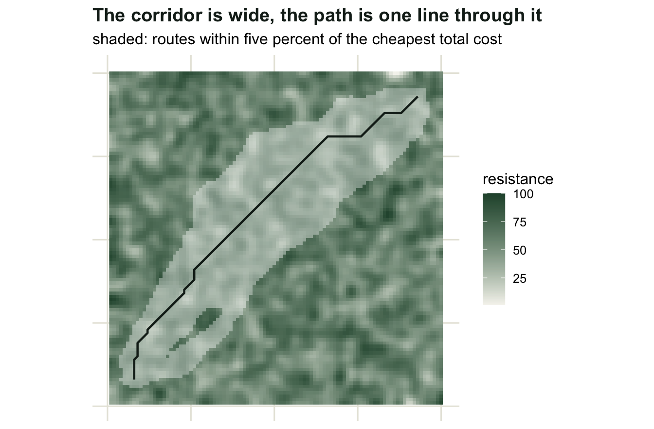

Figure 1: Resistance surface at a contrast of one hundred, with the corridor of routes within five percent of the cheapest total cost shaded and the least-cost path drawn.

How stable is the route?

If the resistance values are guesses, the question is whether the route survives changing them. Compare the sets of cells the paths occupy, using the share of cells shared between two paths out of the cells in either.

overlap <- function(a, b) length(intersect(a, b)) / length(union(a, b))
cat("path overlap, contrast 5 against 1000:",
    round(overlap(runs[[1]]$path, runs[[4]]$path), 4), "\n")

path overlap, contrast 5 against 1000: 0.1557 

cat("contrast 20 against 100:",
    round(overlap(runs[[2]]$path, runs[[3]]$path), 4),
    " contrast 100 against 1000:",
    round(overlap(runs[[3]]$path, runs[[4]]$path), 4), "\n")

contrast 20 against 100: 1  contrast 100 against 1000: 0.9612 

cat("mean resistance along the path at contrast 100:",
    round(mean(runs[[3]]$res[runs[[3]]$path]), 3),
    " over the whole map:", round(mean(runs[[3]]$res), 3), "\n")

mean resistance along the path at contrast 100: 53.512  over the whole map: 58.272 

The path at a contrast of five shares only 15.57 percent of its cells with the path at a contrast of a thousand: same landscape, same endpoints, same ranking of habitat quality, and a substantially different route. Between contrasts of twenty and a hundred the overlap is complete, and between a hundred and a thousand it is 96.12 percent, so the instability is concentrated at low contrast, where the path is nearly a straight line, and the route stabilises once the resistance differences are large enough to be worth a detour.

The last line explains why the saving was small. The mean resistance along the chosen path is 53.512 against 58.272 over the whole map: the least-cost route is only mildly better than average terrain, because on a smooth surface it cannot avoid crossing some expensive ground.

qual_df <- data.frame(x = rep(seq_len(n), each = n),
                      y = rep(seq_len(n), times = n),
                      quality = as.vector(quality))
paths_df <- do.call(rbind, lapply(c(1, 4), function(k) {
  p <- runs[[k]]$path
  data.frame(y = ((p - 1) %% n) + 1, x = ((p - 1) %/% n) + 1,
             contrast = paste("max resistance", runs[[k]]$rmax))
}))

ggplot(qual_df, aes(x, y)) +
  geom_raster(aes(fill = quality)) +
  geom_path(data = paths_df, aes(colour = contrast), linewidth = 0.9) +
  coord_equal() +
  scale_fill_gradient(low = te_pal$forest, high = te_pal$paper,
                      name = "habitat quality") +
  scale_colour_manual(values = c(te_pal$clay, te_pal$ink), name = NULL) +
  labs(title = "The same landscape, two routes",
       subtitle = "only the contrast between best and worst cell changed",
       x = NULL, y = NULL) +
  theme_te() +
  theme(axis.text = element_blank(), panel.grid = element_blank())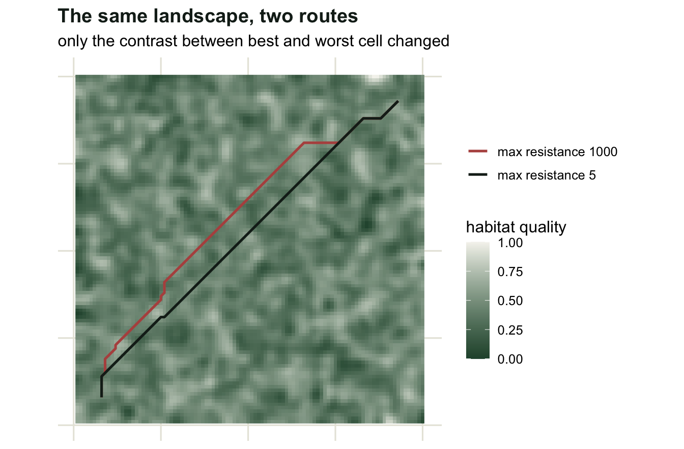

Figure 2: Least-cost paths between the same two points under resistance contrasts of five and one thousand, on the same habitat quality surface.

What this licenses

Three statements are supported by the machinery above, and a fourth is not.

Cost distance is a legitimate, reproducible summary of a resistance surface: given the surface, the numbers are exact and the algorithm has no tuning parameters. It is a good way to compare candidate routes, to rank pairs of patches by isolation, and to produce a corridor map rather than a line.

The corridor map is more honest than the path, because it shows the width of the set of near-optimal routes. Reporting the path alone implies a precision the model does not have, and the measurement above puts a number on that: about a third of this map lies within five percent of the optimum.

The route is sensitive to the contrast of the resistance values, not just to their ranking. That means the standard practice of assigning resistances on an arbitrary scale (one to ten, or one to a hundred) is a modelling decision with consequences, and it should be varied as a sensitivity analysis rather than fixed by convention.

What none of this licenses is the claim that organisms move along the least-cost path. The model optimises total accumulated cost for an omniscient walker; real animals sample locally, take risks, and sometimes cross hostile ground quickly rather than avoiding it. The next tutorial takes the opposite extreme, a walker with no plan at all, and shows that the two models disagree in a way that is itself informative.

References

Adriaensen F, Chardon JP, De Blust G, Swinnen E, Villalba S, Gulinck H, Matthysen E 2003 Landscape and Urban Planning 64(4):233-247 (10.1016/S0169-2046(02)00242-6)

Spear SF, Balkenhol N, Fortin MJ, McRae BH, Scribner K 2010 Molecular Ecology 19(17):3576-3591 (10.1111/j.1365-294X.2010.04657.x)

Sawyer SC, Epps CW, Brashares JS 2011 Journal of Applied Ecology 48(3):668-678 (10.1111/j.1365-2664.2011.01970.x)

Zeller KA, McGarigal K, Whiteley AR 2012 Landscape Ecology 27(6):777-797 (10.1007/s10980-012-9737-0)

Related tutorials

• Patch metrics and fragmentation
• Circuit theory and effective resistance
• Checking a connectivity analysis