library(ggplot2)

te_paper  <- "#f5f4ee"
te_ink    <- "#16241d"
te_body   <- "#2c3a31"
te_forest <- "#275139"
te_rust   <- "#b5534e"
te_gold   <- "#c9b458"
te_line   <- "#dad9ca"

theme_datasheet <- function() {
  theme_minimal(base_size = 12) +
    theme(plot.background  = element_rect(fill = te_paper, colour = NA),
          panel.background = element_rect(fill = te_paper, colour = NA),
          panel.grid.major = element_line(colour = te_line, linewidth = 0.3),
          panel.grid.minor = element_blank(),
          text             = element_text(colour = te_body),
          plot.title       = element_text(colour = te_ink, face = "bold"),
          plot.subtitle    = element_text(colour = te_body),
          axis.text        = element_text(colour = te_body),
          strip.text       = element_text(colour = te_ink))
}Genetic rescue: how many migrants, for how long
R
conservation
population genetics
extinction
simulation
ecology tutorial
Genetic rescue in R: a migrant pulse only delays extinction of an inbred isolate, one a generation holds it off while it lasts, and migrant ancestry runs high.
An island population of wolves, or a panther population cut off by roads and farmland, has been small for long enough that its members are related to one another. Pedigrees show inbreeding coefficients around a fifth, juvenile survival is poor, and the census has been sliding for a decade. Two interventions get discussed. One is to bring in a group of unrelated animals once, as was done when eight female pumas from Texas were released into the Florida panther population. The other is a steady trickle of immigrants, of which Isle Royale received a single natural instalment when one wolf crossed the ice. The textbook number for a trickle is one migrant per generation.
None of the results below is new. Mills and Allendorf reviewed the one migrant per generation rule in 1996 and concluded that one migrant is a desirable minimum that may be inadequate for many natural populations, suggesting between 1 and 10 per generation as a rule of thumb. Hedrick and Fredrickson set out guidelines for genetic rescue from the Florida panther and Mexican wolf programmes, Adams and colleagues traced how the descendants of a single immigrant wolf came to dominate the Isle Royale population, and Whiteley and colleagues reviewed the evidence for genetic rescue and argued that it deserves wider use. What follows is a demonstration of those arguments in a population whose true inbreeding, survival and ancestry are known, so that each claim can be put next to a measured number and the growth rate it depends on.
This site already has the neutral half of the story. Drift, migration and isolation by distance checks the island model equilibrium Fst = 1/(1 + 4Nm) by simulation, under a figure titled “One migrant per generation is the hinge”, but its loci are neutral and nothing dies of inbreeding. Bottlenecks and genetic diversity says in its limits section that its neutral loci say nothing directly about inbreeding depression, and heterozygosity-fitness correlations and power asks whether markers can detect that depression at all. Evolutionary rescue and starting population size is the other kind of rescue: adaptation on a trait in a closed population, with no gene flow. Here inbreeding depression and a population ceiling go into one small isolate, and the post measures what a given schedule of migrants buys against extinction, how that depends on the growth rate, what happens when the migrants stop, and how much of the resident genome is replaced compared with the neutral expectation.
An inbred isolate of thirty
The model is individual-based with discrete generations. The isolate starts with 30 adults, every pair related by a kinship of 0.2 and every adult inbred to the same degree, which is what a long history of small size leaves behind. Each generation the adults produce a Poisson number of offspring with mean 1.6 per adult, each offspring drawing a random mother and a random father from the adults (so some pairs contribute several offspring and some none). An offspring’s inbreeding coefficient is the kinship of its parents, and it survives to breed with probability 0.8 exp(-B F), the usual exponential model of inbreeding depression with B lethal equivalents. At most 30 survivors are kept, chosen at random. The population is counted extinct when fewer than two offspring survive, when the adults are all of one sex, or when fewer than two offspring are born.
Migrants arrive as adults just before breeding. They are unrelated to the residents and to each other and are not inbred, so a migrant crossed with a resident produces an offspring with F of zero. Kinship is carried forward by the tabular rule: the kinship of two offspring is the mean of the four kinships between their parents, and an offspring’s kinship with itself is (1 + F)/2. Each animal also carries a migrant ancestry fraction, one for a migrant, zero for a founder resident and the mean of its parents’ fractions otherwise. These constants were fixed before the first run, and the main cell uses B = 1.5 over 20 generations.
F0     <- 0.2    # starting inbreeding, and kinship among residents
s0     <- 0.8    # survival of an outbred offspring
K_main <- 30     # ceiling on adults
B_main <- 1.5    # lethal equivalents acting on survival
b_main <- 1.6    # mean offspring per adult (Poisson)
G_main <- 20     # generations
r0_out <- s0 * b_main                        # outbred growth factor
r0_in  <- s0 * b_main * exp(-B_main * F0)    # growth factor at the start

run_rep <- function(K, B, b, sched) {
  G <- length(sched)
  kin <- matrix(F0, K, K); diag(kin) <- (1 + F0) / 2
  anc <- rep(0, K); male <- runif(K) < 0.5
  a_tr <- rep(NA_real_, G); an_tr <- a_tr; f_tr <- a_tr; n_tr <- a_tr
  a_neu <- 0; ext <- NA_integer_
  for (g in seq_len(G)) {
    m <- sched[g]
    if (m > 0) {
      n0 <- length(anc)
      kin_new <- matrix(0, n0 + m, n0 + m)
      kin_new[1:n0, 1:n0] <- kin
      diag(kin_new)[n0 + 1:m] <- 0.5
      kin <- kin_new
      anc <- c(anc, rep(1, m)); male <- c(male, runif(m) < 0.5)
      a_neu <- (n0 * a_neu + m) / (n0 + m)
    }
    n_off <- rpois(1, b * length(anc))
    if (!any(male) || all(male) || n_off < 2) { ext <- g; break }
    fem <- which(!male); mal <- which(male)
    dam  <- fem[sample.int(length(fem), n_off, TRUE)]
    sire <- mal[sample.int(length(mal), n_off, TRUE)]
    f_off <- kin[cbind(dam, sire)]
    alive <- which(runif(n_off) < s0 * exp(-B * f_off))
    if (length(alive) > K) alive <- alive[sample.int(length(alive), K)]
    if (length(alive) < 2) { ext <- g; break }
    dam <- dam[alive]; sire <- sire[alive]
    kin <- 0.25 * (kin[dam, dam] + kin[dam, sire] + kin[sire, dam] + kin[sire, sire])
    diag(kin) <- (1 + f_off[alive]) / 2
    anc <- (anc[dam] + anc[sire]) / 2
    male <- runif(length(alive)) < 0.5
    a_tr[g] <- mean(anc); an_tr[g] <- a_neu
    f_tr[g] <- mean(f_off[alive]); n_tr[g] <- length(alive)
  }
  list(ext = ext, a = a_tr, an = an_tr, f = f_tr, n = n_tr)
}

schedule <- function(strat, G = G_main) {
  switch(strat,
         none    = rep(0, G),
         pulse2  = c(2, rep(0, G - 1)),
         pulse5  = c(5, rep(0, G - 1)),
         pulse10 = c(10, rep(0, G - 1)),
         pulse20 = c(20, rep(0, G - 1)),
         one5    = c(rep(1, 5), rep(0, G - 5)),
         alt     = rep(c(1, 0), length.out = G),
         one     = rep(1, G))
}

sim_cell <- function(n_rep, K, B, b, sched) {
  runs <- lapply(seq_len(n_rep), function(i) run_rep(K, B, b, sched))
  list(ext = vapply(runs, function(x) x$ext, 0L),
       a  = t(vapply(runs, function(x) x$a,  numeric(length(sched)))),
       an = t(vapply(runs, function(x) x$an, numeric(length(sched)))),
       f  = t(vapply(runs, function(x) x$f,  numeric(length(sched)))),
       n  = t(vapply(runs, function(x) x$n,  numeric(length(sched)))))
}
p_ext <- function(cell, by = ncol(cell$a)) mean(!is.na(cell$ext) & cell$ext <= by)
mcse_p <- function(p, n) sqrt(p * (1 - p) / n)
The function also tracks a second ancestry number, an, which is what the migrant share would be under neutrality given the population’s own sizes: each arrival of m migrants into n resident adults moves it to (n a + m)/(n + m). If the migrants’ descendants survive no better than anyone else, the realised ancestry should follow an on average. With a full population of K every generation the recursion reduces to the closed form 1 - (1 - 1/(K + 1))^t for one migrant per generation. Both benchmarks can be checked on a run with no inbreeding depression.
n_rep <- 400
neutral_cf <- function(t, K = K_main) 1 - (1 - 1 / (K + 1))^t
set.seed(4101)
neu <- sim_cell(n_rep, K_main, 0, b_main, schedule("one"))
neu_a5 <- mean(neu$a[, 5]); neu_a20 <- mean(neu$a[, 20])
neu_se20 <- sd(neu$a[, 20]) / sqrt(n_rep)
neu_ext <- p_ext(neu)
neu_n <- mean(neu$n[, 20])
neu_f20 <- mean(neu$f[, 20])
With B = 0 and one migrant a generation, none of the 400 populations went extinct and the adult count averaged 29.8 at generation 20. Migrant ancestry averaged 0.147 at generation 5 against a closed form of 0.151, and 0.483 at generation 20 against 0.481, with a Monte Carlo standard error of 0.004 on the second. The engine does not favour migrants when nothing selects for them. Without depression one migrant a generation holds inbreeding near its starting value of 0.2 rather than lowering it much (mean F among the offspring at generation 20 was 0.190), but it stops it rising: in a population of thirty new kinship builds up about as fast as immigration dilutes it. The grid section below shows how far F climbs in the same isolate without migrants.
Twenty migrants at once or one a generation
With B = 1.5 and a starting F of 0.2, an offspring of two residents survives with probability 0.593 instead of 0.8. At 1.6 offspring per adult an outbred population would grow by a factor of 1.28 a generation, and the inbred isolate starts at 0.948: below replacement, and falling as kinship accumulates. Eight migration schedules were run on it, 400 populations each. Four pulses of 2, 5, 10 and 20 migrants arrive in the first generation; one migrant a generation for the first five generations brings the same five animals as the pulse of 5, spread out; one every second generation brings ten; one every generation brings twenty.
strats <- c("none", "pulse2", "pulse5", "pulse10", "pulse20", "one5", "alt", "one")
strat_lab <- c(none = "no migrants", pulse2 = "pulse of 2", pulse5 = "pulse of 5",
               pulse10 = "pulse of 10", pulse20 = "pulse of 20",
               one5 = "1 a generation for 5", alt = "1 every 2 generations",
               one = "1 a generation")
n_mig <- sapply(strats, function(s) sum(schedule(s)))
set.seed(4102)
main <- lapply(strats, function(s) sim_cell(n_rep, K_main, B_main, b_main, schedule(s)))
names(main) <- strats
main_tab <- data.frame(strat = strats, migrants = n_mig,
  pext = sapply(main, p_ext),
  # median time to extinction from the survival curve: first generation at which
  # at most half the populations are still extant (NA if that never happens)
  med_ext = sapply(main, function(x) {
    alive_g <- vapply(1:G_main, function(g) mean(is.na(x$ext) | x$ext > g), 0)
    if (any(alive_g <= 0.5)) min(which(alive_g <= 0.5)) else NA_real_
  }),
  alive5 = sapply(main, function(x) mean(!is.na(x$a[, 5]))),
  a5 = sapply(main, function(x) mean(x$a[, 5], na.rm = TRUE)),
  an5 = sapply(main, function(x) mean(x$an[, 5], na.rm = TRUE)))
mp <- function(s, col) main_tab[main_tab$strat == s, col]
show_tab <- main_tab[, c("migrants", "pext", "med_ext", "a5", "an5")]
rownames(show_tab) <- strat_lab[main_tab$strat]
round(show_tab, 3)
migrants pext med_ext a5 an5
no migrants 0 1.000 11 0.000 0.000
pulse of 2 2 0.990 13 0.095 0.062
pulse of 5 5 0.938 15 0.204 0.143
pulse of 10 10 0.828 17 0.322 0.250
pulse of 20 20 0.623 19 0.462 0.400
1 a generation for 5 5 0.880 16 0.243 0.170
1 every 2 generations 10 0.280 NA 0.165 0.114
1 a generation 20 0.007 NA 0.242 0.171Without migrants the share of populations extinct by generation 20 was 1.000, and the share still extant fell to one half at generation 11. A pulse of 5 left 0.938 extinct and moved that half-way point to generation 15; a pulse of 20, two thirds the size of the resident population, still left 0.623 extinct, with the half-way point at generation 19. The same five migrants spread over five generations did slightly better than the pulse of five, 0.880 extinct, but not differently in kind. One migrant every second generation, ten animals in all, left 0.280 extinct, against 0.828 for the same ten in one pulse. One migrant every generation left 0.007 extinct. With 400 populations per schedule the Monte Carlo standard error of these proportions is at most 0.025.
The comparison that matters is between schedules with the same number of animals. Twenty migrants delivered at once and twenty delivered one a generation differ by 0.62 in the probability of extinction by generation 20. What keeps the isolate going in this model is that migrants keep arriving, more than how many arrive in total. A pulse lowers inbreeding in the first generation of offspring and the benefit then decays as the migrant genomes are shuffled into a population that goes on becoming related to itself.
pers_strats <- c("none", "pulse5", "one5", "pulse10", "alt", "pulse20", "one")
pers <- do.call(rbind, lapply(pers_strats, function(s) {
  ext_s <- main[[s]]$ext
  data.frame(strat = s, generation = 0:G_main,
             alive = vapply(0:G_main, function(g) mean(is.na(ext_s) | ext_s > g), 0))
}))
pers$total <- factor(n_mig[pers$strat], levels = c(0, 5, 10, 20),
                     labels = c("none", "5 migrants", "10 migrants", "20 migrants"))
pers$delivery <- ifelse(grepl("pulse", pers$strat), "one pulse",
                        ifelse(pers$strat == "none", "none", "spread out"))
te_grey <- "#8a9189"
total_cols <- c("none" = te_grey, "5 migrants" = te_rust,
                "10 migrants" = te_gold, "20 migrants" = te_forest)
end_lab <- pers[pers$generation == G_main, ]
end_lab$lab <- strat_lab[end_lab$strat]
end_lab <- end_lab[order(end_lab$alive), ]
end_lab$y_lab <- end_lab$alive
for (i in 2:nrow(end_lab)) {
  end_lab$y_lab[i] <- max(end_lab$y_lab[i], end_lab$y_lab[i - 1] + 0.05)
}
p_pers <- ggplot(pers, aes(generation, alive, colour = total, linetype = delivery,
                           group = strat)) +
  geom_step(linewidth = 0.9) +
  geom_text(data = end_lab, aes(x = G_main + 0.3, y = y_lab, label = lab), hjust = 0,
            size = 3.1, show.legend = FALSE) +
  scale_colour_manual(values = total_cols, name = NULL) +
  scale_linetype_manual(values = c("none" = "solid", "one pulse" = "22",
                                   "spread out" = "solid"), guide = "none") +
  scale_x_continuous(breaks = seq(0, 20, 5), expand = expansion(mult = c(0.02, 0))) +
  scale_y_continuous(breaks = seq(0, 1, 0.25)) +
  coord_cartesian(xlim = c(0, 26.5), ylim = c(0, 1.02), clip = "off") +
  labs(x = "generation", y = "share of populations extant",
       title = "Pulses delay, a trickle holds",
       subtitle = "dashed: all at once; solid: spread over generations") +
  theme_datasheet() +
  theme(legend.position = "bottom")
p_pers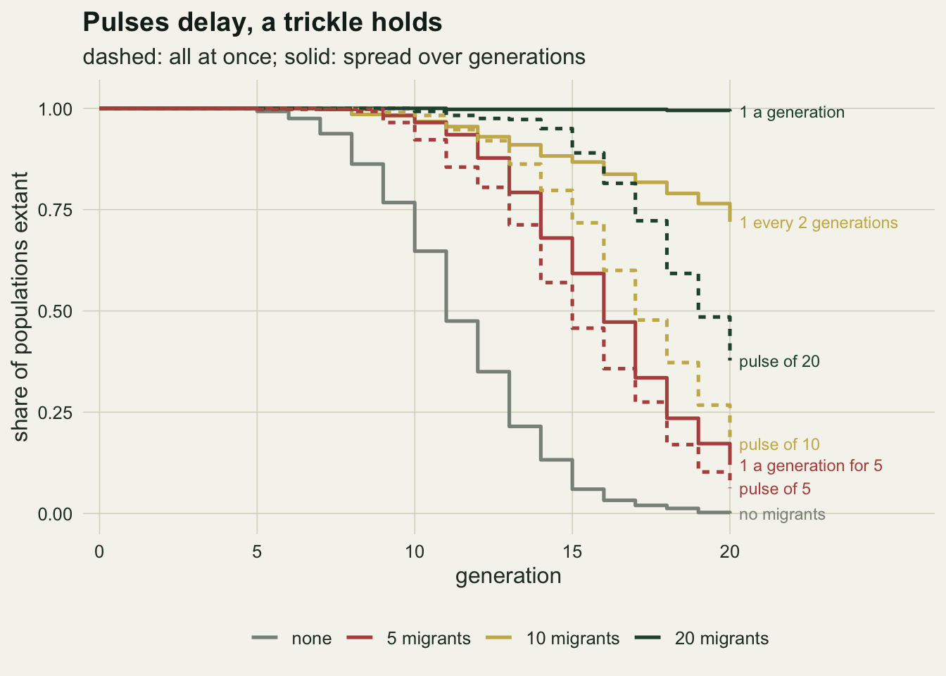
The contrast depends on the growth rate
Every number above is conditional on 1.6 offspring per adult, and no field study knows its fecundity to that precision. The same schedules were run over a range of 1.3 to 1.9 offspring per adult, which puts the outbred growth factor between 1.04 and 1.52, and the starting factor of the inbred isolate between 0.77 and 1.13, so at the top of the range the isolate starts above replacement. Each cell has 300 populations.
b_grid <- seq(1.3, 1.9, by = 0.1)
g_strats <- c("none", "pulse5", "pulse20", "one5", "alt", "one")
n_grid <- 300
set.seed(4103)
growth <- do.call(rbind, lapply(b_grid, function(bb) do.call(rbind, lapply(g_strats, function(s) {
  cell <- sim_cell(n_grid, K_main, B_main, bb, schedule(s))
  data.frame(b = bb, strat = s, pext = p_ext(cell),
             alive5 = mean(!is.na(cell$a[, 5])),
             a5 = mean(cell$a[, 5], na.rm = TRUE), an5 = mean(cell$an[, 5], na.rm = TRUE))
}))))
gp <- function(bb, s, col) growth[abs(growth$b - bb) < 1e-9 & growth$strat == s, col]
At the lowest fecundity, an outbred growth factor of 1.04, one migrant a generation left 0.553 of the populations extinct by generation 20 and every other schedule left at least 0.983. At the highest, 1.52, even the isolate with no migrants survived 20 generations in 0.303 of runs, and a pulse of 5 left only 0.220 extinct. The pulse of 20 against one a generation, the same animals, is the cleanest contrast: 0.913 against 0.087 at 1.5 offspring per adult, 0.300 against 0.007 at 1.7, and 0.040 against 0.000 at 1.9. A single headline probability of extinction under one migrant per generation would therefore mean little: across this range it runs from 0.553 to 0.000. One migrant a generation had the lowest or equal-lowest (within Monte Carlo error) extinction probability at every fecundity tried; what fecundity changes is the size of every gap. A twenty generation horizon also hides the difference between a population that is safe and one that is only being held up, which the section on duration takes up.
growth$total <- factor(n_mig[growth$strat], levels = c(0, 5, 10, 20),
                       labels = c("none", "5 migrants", "10 migrants", "20 migrants"))
growth$delivery <- ifelse(grepl("pulse", growth$strat), "one pulse",
                          ifelse(growth$strat == "none", "none", "spread out"))
growth$se <- mcse_p(growth$pext, n_grid)
ggplot(growth, aes(s0 * b, pext, colour = total, linetype = delivery, group = strat)) +
  geom_line(linewidth = 0.9) +
  geom_errorbar(aes(ymin = pext - 2 * se, ymax = pext + 2 * se),
                width = 0, linewidth = 0.4, linetype = "solid") +
  geom_point(size = 1.9) +
  scale_colour_manual(values = total_cols, name = NULL) +
  scale_linetype_manual(values = c("none" = "solid", "one pulse" = "22",
                                   "spread out" = "solid"), guide = "none") +
  scale_x_continuous(breaks = s0 * b_grid, labels = sprintf("%.2f", s0 * b_grid)) +
  labs(x = "outbred growth factor per generation", y = "P(extinct by generation 20)",
       title = "Fecundity sets the size of every gap",
       subtitle = "dashed: one pulse; solid: spread out; bars: two Monte Carlo standard errors") +
  theme_datasheet() +
  theme(legend.position = "bottom")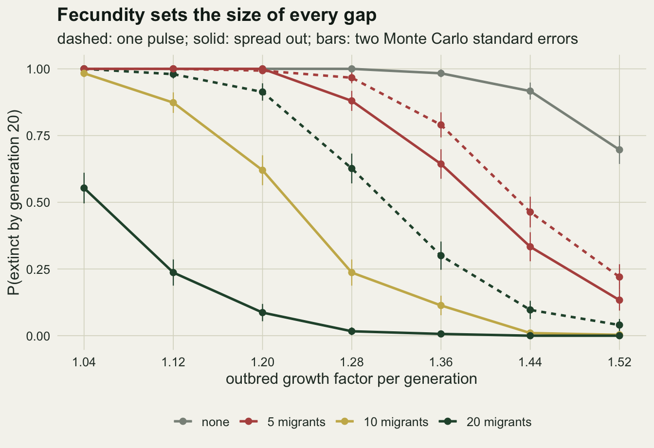
The strength of inbreeding depression and the ceiling on population size matter in the same way. The next grid holds fecundity at 1.6 and varies B over 0, 0.75, 1.5 and 3 and K over 20, 30 and 60, for no migrants, a pulse of 5 and one migrant a generation.
K_grid <- c(20, 30, 60); B_grid <- c(0, 0.75, 1.5, 3)
set.seed(4104)
kb <- do.call(rbind, lapply(K_grid, function(KK) do.call(rbind, lapply(B_grid, function(BB)
  do.call(rbind, lapply(c("none", "pulse5", "one"), function(s) {
    cell <- sim_cell(n_grid, KK, BB, b_main, schedule(s))
    data.frame(K = KK, B = BB, strat = s, pext = p_ext(cell),
               f20 = mean(cell$f[, 20], na.rm = TRUE))
  }))))))
kp <- function(KK, BB, s) kb$pext[kb$K == KK & kb$B == BB & kb$strat == s]
b0_max <- max(kb$pext[kb$B == 0])
b3_other_min <- min(kb$pext[kb$B == 3 & kb$strat != "one"])
kf <- function(KK, BB, s) kb$f20[kb$K == KK & kb$B == BB & kb$strat == s]
With no inbreeding depression the largest extinction probability in any schedule at any size was 0.000, which is the check that extinction here is driven by inbreeding and not by demographic noise at 1.6 offspring per adult. The same B = 0 runs show what the trickle does to inbreeding: at K = 30 mean F among the offspring at generation 20 was 0.425 with no migrants, 0.385 after a pulse of 5 and 0.191 with one migrant a generation, so the trickle prevents a large rise rather than bringing F down. At B = 0.75 the isolate without migrants lost 0.707 of populations at K = 20, 0.240 at K = 30 and 0.000 at K = 60. At B = 1.5 the pulse of 5 left 0.993, 0.923 and 0.477 extinct across the three ceilings, against 1.000, 0.993 and 0.900 with no migrants: the same five animals buy more in a larger isolate, which also builds up new kinship more slowly on its own. At B = 3 no schedule saved every population: one migrant a generation left 0.450, 0.400 and 0.233 extinct, while under the other two schedules every population went extinct at every ceiling.
kb$strat_lab <- factor(strat_lab[kb$strat], levels = strat_lab[c("none", "pulse5", "one")])
kb$K_lab <- factor(paste("K =", kb$K), levels = paste("K =", K_grid))
ggplot(kb, aes(B, pext, colour = strat_lab)) +
  geom_line(linewidth = 0.9) +
  geom_point(size = 2) +
  facet_wrap(~ K_lab, ncol = 3) +
  scale_colour_manual(values = c("#8a9189", te_rust, te_forest), name = NULL) +
  scale_x_continuous(breaks = B_grid, labels = c("0", "0.75", "1.5", "3")) +
  labs(x = "lethal equivalents B", y = "P(extinct by generation 20)",
       title = "Depression and size, three schedules") +
  theme_datasheet() +
  theme(legend.position = "bottom", panel.spacing.x = unit(1.2, "lines"))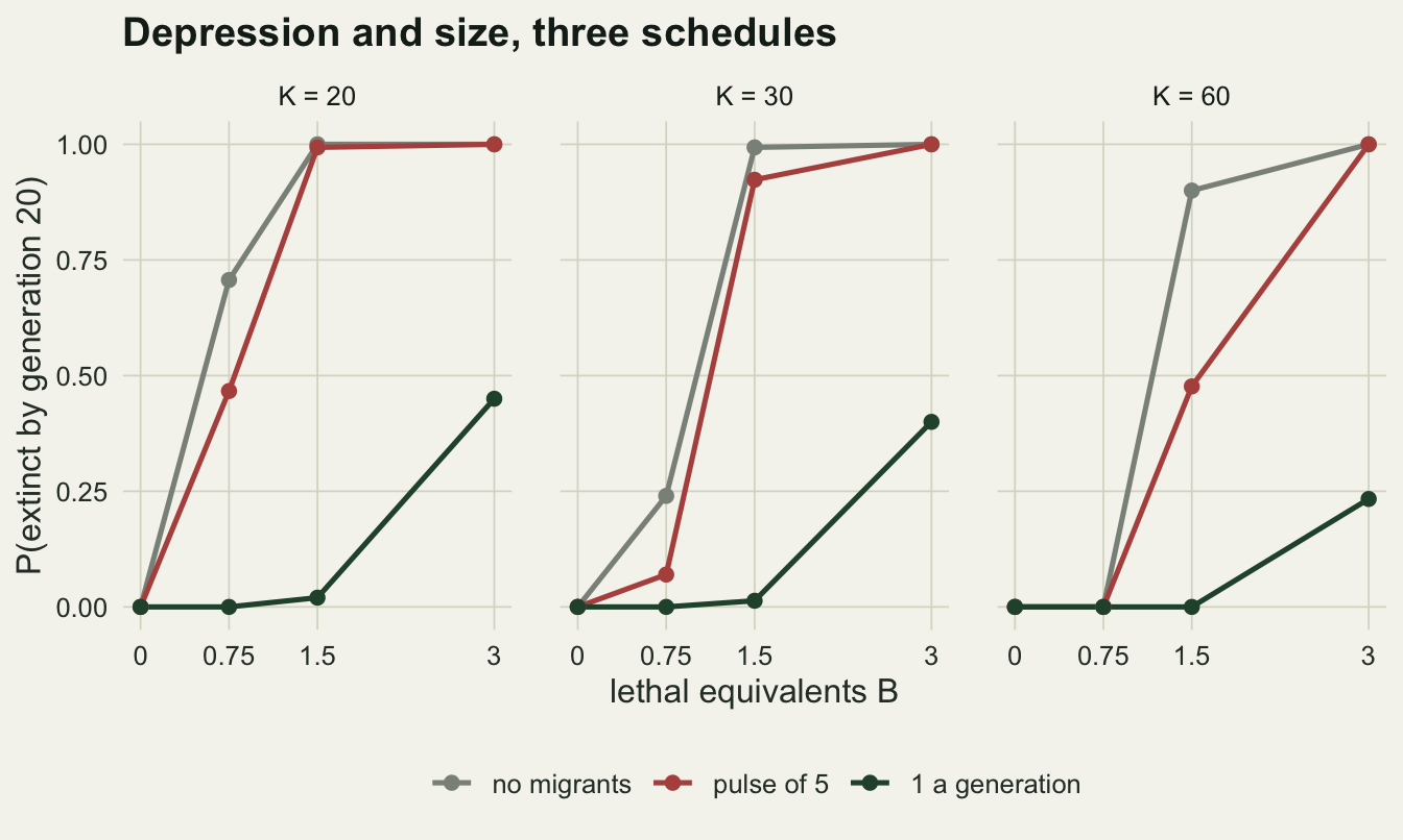
For how long
A rescue plan is usually written as a number of animals. The results above suggest it should be written as a duration, so the next run extends the horizon to 40 generations and stops the one migrant a generation after 0, 5, 10, 20, 30 or all 40 generations, at 1.6 and 1.8 offspring per adult.
G_long <- 40; t_grid <- c(0, 5, 10, 20, 30, 40); b_dur <- c(1.6, 1.8)
set.seed(4105)
dur <- do.call(rbind, lapply(b_dur, function(bb) do.call(rbind, lapply(t_grid, function(tt) {
  cell <- sim_cell(n_grid, K_main, B_main, bb, c(rep(1, tt), rep(0, G_long - tt)))
  data.frame(b = bb, T = tt, p20 = p_ext(cell, 20), p40 = p_ext(cell, 40),
             med = median(cell$ext, na.rm = TRUE), f_stop = if (tt > 0) mean(cell$f[, tt], na.rm = TRUE) else NA_real_)
}))))
dp <- function(bb, tt, col) dur[dur$b == bb & dur$T == tt, col]
At 1.6 offspring per adult, a trickle that ran for 20 generations left a share of 0.000 extinct at generation 20, the moment it stopped, and 0.990 by generation 40. Their median extinction generation was 32, 12 generations after the last migrant, which is close to the 11 generations an isolate with no migrants lasts from the start. Mean F among the surviving offspring at the generation the migrants stopped was 0.141, against 0.2 at the start. An offspring with that inbreeding coefficient survives with probability 0.648, which at 1.6 offspring per adult is a growth factor of 1.037: barely above replacement, with nothing left to stop kinship from building up again once the migrants stop. Only the trickle that never stopped kept extinction by generation 40 down to 0.030. At 1.8 offspring per adult the picture is gentler but the same: stopping after 20 generations gave 0.697 extinct by generation 40, stopping after 30 gave 0.013, but that horizon ends only ten generations after the stop, fewer than the median lifetime of 16 generations for an isolate with no migrants at that fecundity.
So in this model one migrant per generation does not rescue the isolate in the sense of leaving it able to persist alone. It holds the population at a level where it replaces itself for as long as the migrants keep coming. That is not a flaw in the rule; the rule was derived to keep a small population from diverging and losing variation by drift, and it is doing that. A population that is to stand on its own afterwards needs something the model does not have: room to grow, so that new kinship accumulates slowly, or purging of the deleterious alleles behind B.
dur$b_lab <- factor(sprintf("%.1f offspring per adult", dur$b))
ggplot(dur, aes(T, p40, colour = b_lab)) +
  geom_line(linewidth = 0.9) +
  geom_point(size = 2.2) +
  scale_colour_manual(values = c(te_rust, te_forest), name = NULL) +
  scale_x_continuous(breaks = t_grid) +
  scale_y_continuous(limits = c(0, 1)) +
  labs(x = "generations of one migrant a generation, then none",
       y = "P(extinct by generation 40)",
       title = "Stopping the trickle restarts the clock") +
  theme_datasheet() +
  theme(legend.position = "bottom")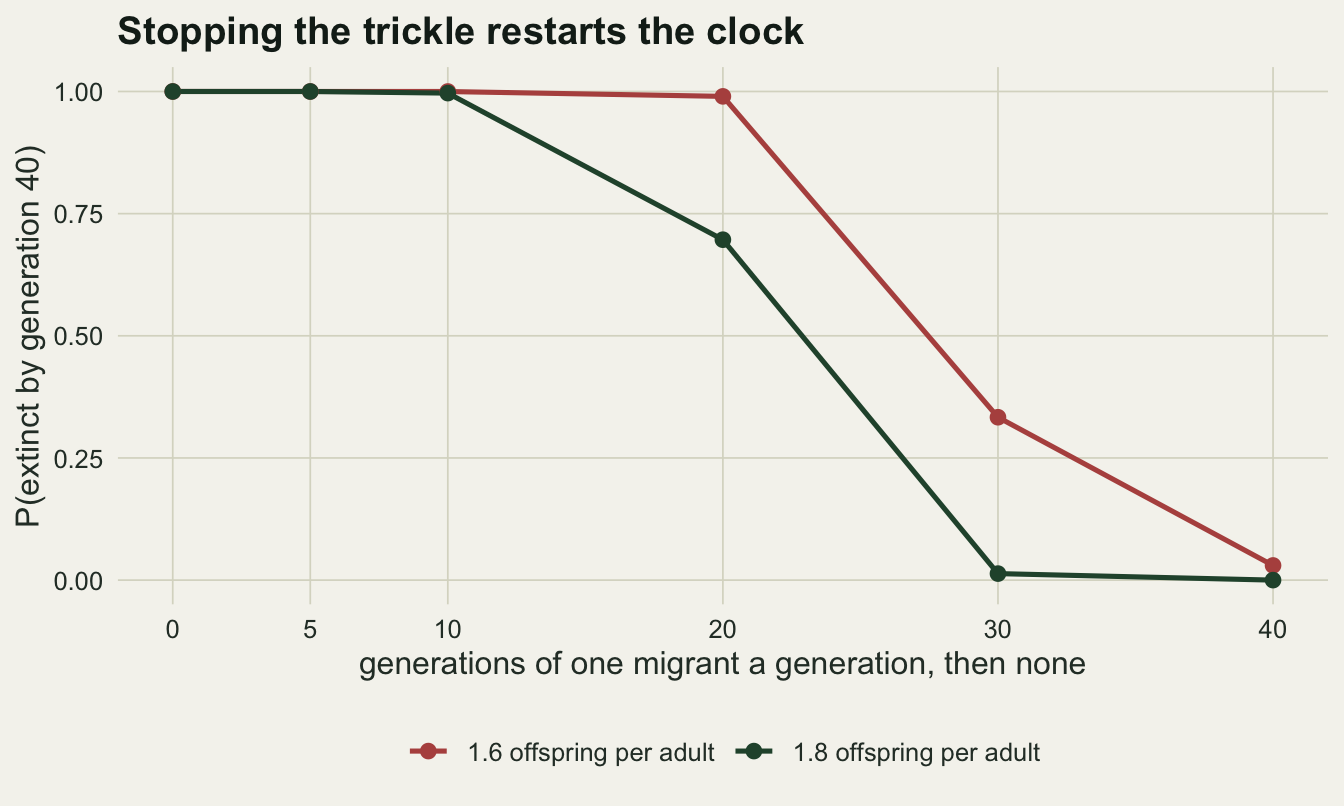
How much of the resident genome goes
The price of rescue is ancestry. If the migrants’ descendants survive better than residents because they are less inbred, the migrant share of the genome rises faster than the neutral calculation says, and in a population rescued this way the resident genome can be largely replaced. Measuring that excess has a trap in it: a population that went extinct has no ancestry to average, so an average over surviving populations at generation 20 compares a selected subset with a benchmark that assumes nothing was selected. The unconditional version is ancestry at a fixed early generation at which (nearly) every population is still alive, averaged over all of them. In the main cell the share alive at generation 5 was at least 0.993 for every schedule.
b_low <- 1.35
set.seed(4106)
low <- sim_cell(n_rep, K_main, B_main, b_low, schedule("one"))
surv <- is.na(low$ext)
low_p <- mean(!surv)
low_a5_s <- mean(low$a[surv, 5]); low_a5_e <- mean(low$a[!surv, 5], na.rm = TRUE)
low_se_diff <- sqrt(var(low$a[surv, 5]) / sum(surv) + var(low$a[!surv, 5], na.rm = TRUE) / sum(!is.na(low$a[!surv, 5])))
low_a20 <- mean(low$a[surv, 20]); low_an20 <- mean(low$an[surv, 20])
low_n <- mean(low$n[surv, 10:20])
one <- main$one
one_a20 <- mean(one$a[, 20], na.rm = TRUE); one_an20 <- mean(one$an[, 20], na.rm = TRUE)
At generation 5 under one migrant a generation, migrant ancestry averaged 0.242 over all 400 populations. The closed form for a full population of 30 gives 0.151, and the size-matched neutral recursion, which uses each population’s own adult counts, gives 0.171. The gap to the closed form, 0.091, splits into 0.020 that comes from the populations being smaller than 30, so one migrant is a larger share, and 0.071 that comes from the migrants’ descendants surviving better. For the pulse of 5 there is no size component, because the pulse arrives into a full population and the neutral share is exactly 5/35 = 0.143; the realised share at generation 5 was 0.204. Across the fecundity range of the previous section, the selection part under one migrant a generation ran from 0.060 to 0.078, larger where growth was lower and inbred offspring were more often the ones to die.
By generation 20 the same populations had a migrant share of 0.702, against 0.560 from the size-matched recursion and 0.481 from the closed form, averaged over the 0.993 share that survived. At 1.6 offspring per adult so few populations died that the conditioning hardly matters. At 1.35 offspring per adult it does: 0.400 of populations were extinct by generation 20, and the survivors carried a migrant share of 0.899. Set against the closed form of 0.481 that looks like strong selection for migrant genes. Against the size-matched recursion for the same survivors, 0.808, most of it is not: the survivors were small, averaging 11.0 adults over generations 10 to 20, and one migrant into a population of eleven is a large share with no selection at all. Whether the later survivors had already taken up more migrant ancestry by generation 5 was also checked: 0.311 for the populations that went on to survive against 0.294 for those that went extinct, a difference of 0.017 with a standard error of 0.011, so no clear sign that survival was decided by early admixture in this design.
anc_df <- rbind(
  data.frame(generation = 1:G_main, value = colMeans(one$a, na.rm = TRUE),
             series = "simulated, B = 1.5"),
  data.frame(generation = 1:G_main, value = colMeans(one$an, na.rm = TRUE),
             series = "neutral, own sizes (B = 1.5 runs)"),
  data.frame(generation = 1:G_main, value = colMeans(neu$a),
             series = "simulated, B = 0"),
  data.frame(generation = 1:G_main, value = neutral_cf(1:G_main),
             series = "closed form, K = 30"))
anc_df$series <- factor(anc_df$series, levels = unique(anc_df$series))
ggplot(anc_df, aes(generation, value, colour = series, linetype = series)) +
  geom_line(linewidth = 0.9) +
  scale_colour_manual(values = c(te_forest, te_gold, te_rust, te_ink), name = NULL) +
  scale_linetype_manual(values = c("solid", "solid", "solid", "22"), name = NULL) +
  scale_x_continuous(breaks = c(1, 5, 10, 15, 20)) +
  scale_y_continuous(limits = c(0, 0.8)) +
  labs(x = "generation", y = "mean migrant ancestry",
       title = "Migrant genes outrun the neutral share") +
  guides(colour = guide_legend(nrow = 2), linetype = guide_legend(nrow = 2)) +
  theme_datasheet() +
  theme(legend.position = "bottom")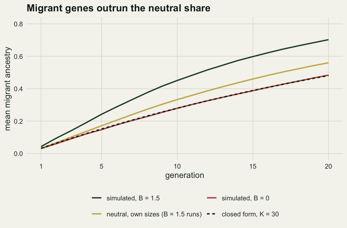
What to report
Give the schedule as a duration as well as a number. In these runs twenty migrants in one pulse left 0.623 of populations extinct by generation 20 and the same twenty spread one a generation left 0.007, and a trickle that stopped after 20 generations left 0.990 extinct 20 generations later. A plan that says “twenty animals” has not said which of these it is.
Report the extinction risk as a range over growth rates, not as one probability. The growth rate is the least known quantity in any small population model and in this one it moved the extinction probability under one migrant a generation from 0.553 to 0.000.
Report migrant ancestry unconditionally, at a fixed generation, together with the share of populations alive then, and set it beside a neutral benchmark that uses the population’s own sizes. The closed form for a full population is a good arithmetic check but a poor benchmark for a population that has been shrinking, because a smaller population takes a larger share from each migrant without any selection.
Report the lethal equivalents assumed and which fitness component they act on. Without migrants, at B = 0.75, an isolate capped at 60 lost 0.000 of its populations and one capped at 20 lost 0.707; at B = 3 even one migrant a generation left between 0.233 and 0.450 extinct.
Honest limits
Inbreeding depression acts on survival only, through a fixed B, with no genotypes. Real depression also hits fecundity and mating success, which would make every schedule look worse, and real deleterious alleles can be purged by the same selection that kills inbred offspring, which would let a population recover some fitness on its own and would make the rescue more durable than the duration section shows. Purging needs explicit loci and was left out to keep the whole model to pedigree kinship.
The migrants are unrelated, outbred and fully compatible. A source population that has diverged can carry outbreeding depression, often showing in the second generation of crosses rather than the first, and that would lower the excess ancestry and could reverse the benefit of a large pulse. No such scenario was run, so the results here are the favourable case for rescue. Nor does the model score the resident genome being replaced as a cost; with local adaptation, a trickle that never stops trades extinction risk for swamping, which is why rescue guidelines monitor migrant ancestry.
The ceiling of 30 is fixed. The best known rescues, such as the Florida panther, were followed by population growth, and a population that doubles after the migrants arrive accumulates new kinship half as fast. The finding that stopping the trickle restarts the extinction clock belongs to a population held small, which is the case the one migrant rule was written for but not the only one managers face.
Mating is random with replacement, generations do not overlap, and migrants breed in the generation they arrive. Long-lived species keep founders and immigrants alive and breeding over several generations, which spreads a pulse out in time, and that makes a pulse look more like a trickle than it does here. Real immigrants may also breed less often than residents in their first seasons.
The extinction probabilities are for a 20 or 40 generation horizon. For a wolf, with a generation time of several years, 20 generations is close to a century, longer than any management plan, but the duration section shows that a short horizon can call a population safe that is only being held up.
References
Mills LS, Allendorf FW 1996 Conservation Biology 10(6):1509-1518 (10.1046/j.1523-1739.1996.10061509.x)
Hedrick PW, Fredrickson R 2010 Conservation Genetics 11(2):615-626 (10.1007/s10592-009-9999-5)
Adams JR, Vucetich LM, Hedrick PW, Peterson RO, Vucetich JA 2011 Proceedings of the Royal Society B 278(1723):3336-3344 (10.1098/rspb.2011.0261)
Whiteley AR, Fitzpatrick SW, Funk WC, Tallmon DA 2015 Trends in Ecology and Evolution 30(1):42-49 (10.1016/j.tree.2014.10.009)