library(ggplot2)
library(patchwork)

te_paper  <- "#f5f4ee"
te_ink    <- "#16241d"
te_body   <- "#2c3a31"
te_forest <- "#275139"
te_rust   <- "#b5534e"
te_gold   <- "#c9b458"
te_line   <- "#dad9ca"
te_sage   <- "#7fa98a"

theme_datasheet <- function() {
  theme_minimal(base_size = 12) +
    theme(plot.background  = element_rect(fill = te_paper, colour = NA),
          panel.background = element_rect(fill = te_paper, colour = NA),
          panel.grid.major = element_line(colour = te_line, linewidth = 0.3),
          panel.grid.minor = element_blank(),
          text             = element_text(colour = te_body),
          plot.title       = element_text(colour = te_ink, face = "bold"),
          plot.subtitle    = element_text(colour = te_body),
          axis.text        = element_text(colour = te_body))
}Heterozygosity-fitness correlations and power
R
population genetics
inbreeding
statistical power
simulation
ecology tutorial
Simulate heterozygosity-fitness correlations in R: how often a dozen microsatellites detect real inbreeding depression, and what the g2 test can and cannot say.
An island population of songbirds has been ringed for years, and one season’s nestlings have blood samples and a known fate: each chick either recruited into the breeding population or did not. The laboratory types twelve microsatellites on every chick. The question on the grant is whether inbred chicks survive less well, and there is no pedigree deep enough to give each chick an inbreeding coefficient. So the analysis uses the markers instead. Each chick gets a multilocus heterozygosity, the share of its loci that are heterozygous, survival is regressed on it, and the slope is the heterozygosity-fitness correlation, the HFC.
The logic is sound. An inbred individual carries more of its genome identical by descent, identical by descent loci are homozygous, so inbred individuals are less heterozygous at neutral markers as well as at the genes that matter for survival. The weakness is in the word “less”. Twelve loci are a small sample of a genome, and whether a given chick happens to be heterozygous at a given marker depends far more on allele frequencies than on its inbreeding. The markers see inbreeding through a keyhole.
This post sits between three existing ones. Bottlenecks and genetic diversity ends with the warning that its neutral loci “say nothing directly about inbreeding depression”; the HFC is the field method that tries to make them say something. Hardy-Weinberg expectations in R shows that a heterozygote deficit is weak evidence of inbreeding in a population sample; here the question is the individual level version, whether one animal’s heterozygosity tells us its inbreeding. And measurement error and regression dilution shows how a noisy predictor flattens a slope in proportion to its reliability. Heterozygosity is a noisy predictor of inbreeding, and its reliability has a name in this literature: it is set by the identity disequilibrium statistic g2 and by the number of loci.
The post builds the simulation, implements g2 exactly as David and colleagues (2007) define it and checks it against a brute force version, prints the closed forms that Szulkin, Bierne and David (2010) give for the correlations as arithmetic checks, and then measures the two things the closed forms do not give: how often an HFC test detects real inbreeding depression, and how often the g2 test, which is meant to show that a panel can see inbreeding at all, comes out significant on the same data.
Markers see inbreeding through a keyhole
The generating model is deliberately simple. Each individual has an inbreeding coefficient f drawn from a mixture of pedigree classes: in the main scenario 70 per cent are outbred (f = 0), 20 per cent are offspring of half sibs (f = 0.125) and 10 per cent are offspring of full sibs or parent and offspring (f = 0.25). At every marker locus, independently, the two copies are identical by descent with probability f, in which case the individual is homozygous. Otherwise it is heterozygous with the locus’s expected heterozygosity, 0.7 for a microsatellite and 2p(1 - p) for a SNP with minor allele frequency p. Three per cent of genotypes are missing at random, as they are in any real panel.
Survival is Bernoulli with a logit that falls by 6 units per unit of f from an outbred survival of 0.6. The markers are neutral; they relate to survival only through f. This is the “general effect” case of the HFC literature, the one in which the markers are genuine proxies for genome wide inbreeding.
Multilocus heterozygosity is computed as the standardised heterozygosity (sMLH) of Coltman and colleagues (1999), as the inbreedR package implements it: the proportion of an individual’s typed loci that are heterozygous, divided by the mean heterozygosity in the sample of those same loci. Missing loci and uneven locus diversity then do not change the scale, and every heterozygous locus counts the same, whatever its diversity.
make_panel <- function(n_ind, het, fprob, fval, miss = 0.03) {
  n_loc <- length(het)
  f_ind <- fval[sample.int(length(fval), n_ind, replace = TRUE, prob = fprob)]
  ibd   <- runif(n_ind * n_loc) < f_ind
  is_het <- (runif(n_ind * n_loc) < rep(het, each = n_ind)) & !ibd
  typed <- runif(n_ind * n_loc) >= miss
  h0 <- matrix(is_het & typed, n_ind, n_loc) * 1
  tt <- matrix(typed, n_ind, n_loc) * 1
  poly <- colSums(h0) > 0                  # drop loci with no heterozygote
  h0 <- h0[, poly, drop = FALSE]; tt <- tt[, poly, drop = FALSE]
  loc_mean <- colSums(h0) / colSums(tt)
  # Coltman et al. (1999) sMLH, as in inbreedR::sMLH
  smlh <- (rowSums(h0) / rowSums(tt)) / as.vector(tt %*% loc_mean / rowSums(tt))
  list(f = f_ind, h0 = h0, tt = tt, smlh = smlh)
}

surv_int   <- qlogis(0.6)
surv_slope <- -6
het_ms     <- 0.7
set.seed(4412)
maf_snp <- runif(100, 0.05, 0.5)
panels <- list("12 microsatellites" = rep(het_ms, 12),
               "30 microsatellites" = rep(het_ms, 30),
               "100 SNPs"           = 2 * maf_snp * (1 - maf_snp))
scenarios <- list(
  "no variance in f"     = list(p = 1, v = 0),
  "pedigree mixture"     = list(p = c(0.7, 0.2, 0.1), v = c(0, 0.125, 0.25)),
  "rare close inbreeding" = list(p = c(0.95, 0.05), v = c(0, 0.25)))

f_mean  <- sum(scenarios[[2]]$p * scenarios[[2]]$v)
f_var   <- sum(scenarios[[2]]$p * scenarios[[2]]$v^2) - f_mean^2
g2_true <- f_var / (1 - f_mean)^2
surv_fs <- plogis(surv_int + surv_slope * 0.25)

set.seed(1907)
demo_ms  <- make_panel(200, panels[[1]], scenarios[[2]]$p, scenarios[[2]]$v)
demo_snp <- make_panel(200, panels[[3]], scenarios[[2]]$p, scenarios[[2]]$v)
r_demo_ms  <- cor(demo_ms$smlh, demo_ms$f)
r_demo_snp <- cor(demo_snp$smlh, demo_snp$f)
q_ms <- tapply(demo_ms$smlh, demo_ms$f, median)
overlap_ms <- mean(demo_ms$smlh[demo_ms$f == 0.25] >
                   median(demo_ms$smlh[demo_ms$f == 0]))
The expected survival of a full sib offspring is 0.25, a strong inbreeding effect. In one simulated season of 200 chicks typed at 12 microsatellites, the correlation between sMLH and true f is -0.32. The median sMLH is 1.02 for outbred chicks and 0.82 for full sib offspring, so the classes do differ, and still 17 per cent of the full sib offspring are more heterozygous than the median outbred chick. With 100 SNPs on a different simulated season the correlation is -0.52.
keyhole_df <- rbind(
  data.frame(f = demo_ms$f, smlh = demo_ms$smlh, panel = "12 microsatellites"),
  data.frame(f = demo_snp$f, smlh = demo_snp$smlh, panel = "100 SNPs"))
keyhole_df$panel <- factor(keyhole_df$panel, levels = c("12 microsatellites", "100 SNPs"))
keyhole_df$f_lab <- factor(sprintf("%.3f", keyhole_df$f))

ggplot(keyhole_df, aes(f_lab, smlh)) +
  geom_jitter(width = 0.18, height = 0, colour = te_forest, alpha = 0.45, size = 1.4) +
  geom_boxplot(fill = NA, colour = te_ink, outlier.shape = NA, width = 0.5,
               linewidth = 0.5) +
  facet_wrap(~ panel) +
  labs(x = "pedigree inbreeding coefficient f", y = "standardised heterozygosity",
       title = "Inbred individuals are less heterozygous, on average",
       subtitle = "the classes overlap widely, more so at twelve loci") +
  theme_datasheet()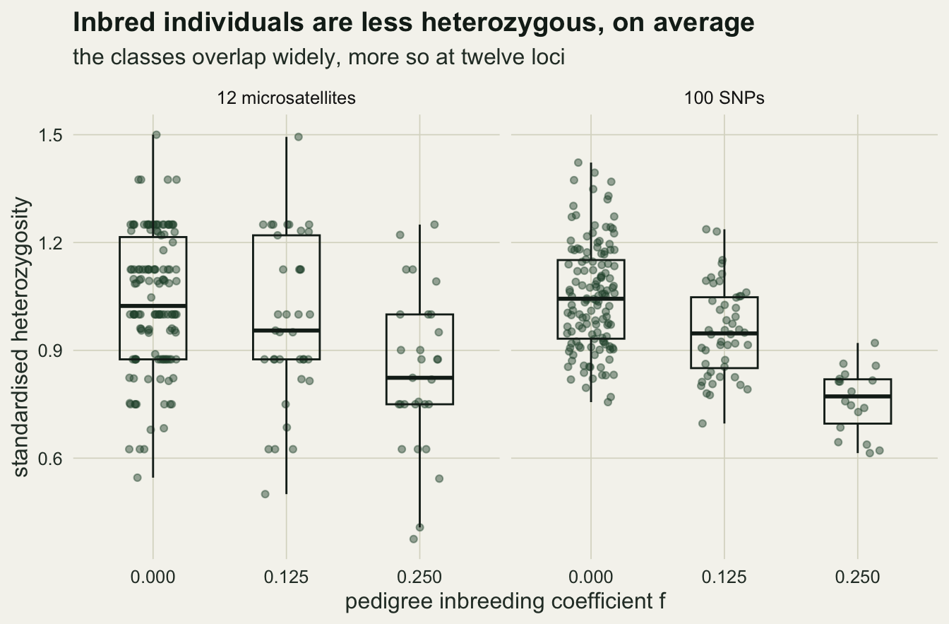
The g2 estimator, exactly
If loci are unlinked, the only thing that makes heterozygosity at one locus predict heterozygosity at another is shared variation in f across individuals. This is called identity disequilibrium, and David and colleagues (2007) measure it by g2, the excess of heterozygosity covariance between loci over what independence would give, scaled by the mean heterozygosities. In the population it equals the variance of f divided by the square of one minus the mean of f. For the pedigree mixture that is 0.00762: small, as it usually is in outcrossing animals, because most individuals in such populations are not very inbred.
David and colleagues (2007) give the estimator used in practice, and it is written to cope with missing genotypes. Code heterozygosity at locus l in individual i as 1 or 0. For each ordered pair of different loci l and l’, the numerator term is the sum over individuals of the product of their heterozygosities at l and l’, divided by the number of individuals typed at both loci. The denominator term is the same product taken over ordered pairs of different individuals i and j (i at l, j at l’), divided by the number of such pairs with i typed at l and j typed at l’. Both terms are summed over all ordered locus pairs, and g2 is the ratio of the two sums minus one. The pair count in the denominator simplifies to (n - 1)(n - m_l - m_l’) + m_l m_l’ - m_ll’, with m_l missing at l and m_ll’ missing at both; this is the form in the inbreedR package of Stoffel and colleagues (2016), which implements the David et al. estimator, and it was used here to check the reading of the definition.
The version below does the same thing with two cross products, which is what makes 99 permutations per study affordable. It is checked against a brute force version that loops over every locus pair and every pair of individuals, on a data set with missing genotypes.
g2_david <- function(h0, tt) {
  p_ll <- crossprod(h0)                    # sum_i h_il h_il'
  c_ll <- crossprod(tt)                    # typed at both
  q_ll <- outer(colSums(h0), colSums(h0)) - p_ll   # sum over i != j
  d_ll <- outer(colSums(tt), colSums(tt)) - c_ll
  num <- sum(p_ll / c_ll) - sum(diag(p_ll) / diag(c_ll))
  den <- sum(q_ll / d_ll) - sum(diag(q_ll) / diag(d_ll))
  num / den - 1
}

g2_brute <- function(h0, tt) {
  n_ind <- nrow(h0); n_loc <- ncol(h0); num <- 0; den <- 0
  for (l1 in seq_len(n_loc)) for (l2 in seq_len(n_loc)) {
    if (l1 == l2) next
    s_same <- 0; n_same <- 0; s_diff <- 0; n_diff <- 0
    for (i in seq_len(n_ind)) {
      if (tt[i, l1] == 1 && tt[i, l2] == 1) {
        s_same <- s_same + h0[i, l1] * h0[i, l2]; n_same <- n_same + 1
      }
      for (j in seq_len(n_ind)) {
        if (j != i && tt[i, l1] == 1 && tt[j, l2] == 1) {
          s_diff <- s_diff + h0[i, l1] * h0[j, l2]; n_diff <- n_diff + 1
        }
      }
    }
    num <- num + s_same / n_same; den <- den + s_diff / n_diff
  }
  num / den - 1
}

sub_rows <- 1:60
g2_fast_sub  <- g2_david(demo_ms$h0[sub_rows, ], demo_ms$tt[sub_rows, ])
g2_brute_sub <- g2_brute(demo_ms$h0[sub_rows, ], demo_ms$tt[sub_rows, ])
n_miss_sub   <- sum(demo_ms$tt[sub_rows, ] == 0)

g2_perm_p <- function(h0, tt, n_perm = 99) {
  n_ind <- nrow(h0); n_loc <- ncol(h0)
  key <- rep(seq_len(n_loc), each = n_ind)
  g2_obs <- g2_david(h0, tt); n_ge <- 0
  for (k in seq_len(n_perm)) {             # shuffle each locus across individuals
    o <- order(key + runif(n_ind * n_loc), method = "radix")
    n_ge <- n_ge + (g2_david(matrix(h0[o], n_ind, n_loc),
                             matrix(tt[o], n_ind, n_loc)) >= g2_obs)
  }
  c(g2 = g2_obs, p = (1 + n_ge) / (n_perm + 1))
}
set.seed(77)
demo_test <- g2_perm_p(demo_ms$h0, demo_ms$tt)
n_boot <- 199
boot_g2 <- replicate(n_boot, {
  rows <- sample.int(nrow(demo_ms$h0), replace = TRUE)
  g2_david(demo_ms$h0[rows, ], demo_ms$tt[rows, ])
})
boot_ci <- quantile(boot_g2, c(0.025, 0.975))
On the first 60 individuals, with 25 missing genotypes, the matrix version gives -0.0031906307 and the loop gives -0.0031906307. On all 200 chicks the estimate is 0.00261 against the population value 0.00762, and the permutation test, which shuffles each locus independently across individuals to destroy identity disequilibrium while keeping every locus’s heterozygosity, gives p = 0.31 from 99 permutations. A bootstrap over individuals (199 resamples) gives a 95 per cent interval from -0.00541 to 0.01268.
Sixty studies per cell
The grid crosses the three panels with the three inbreeding scenarios at 200 individuals, and adds 100 and 400 individuals for the pedigree mixture. Each cell holds 60 simulated studies. In every study three tests are run at the five per cent level: a logistic regression of survival on true f (the benchmark nobody in the field has), a logistic regression of survival on sMLH (the HFC), and the g2 permutation test with 99 permutations. With 60 studies a rejection rate has a Monte Carlo standard error of at most 0.065. These design constants were fixed before the grid was run, and the grid is the slow part of the post.
one_study <- function(n_ind, het, sc) {
  pan <- make_panel(n_ind, het, sc$p, sc$v)
  surv <- rbinom(n_ind, 1, plogis(surv_int + surv_slope * pan$f))
  has_f <- var(pan$f) > 0
  p_hfc <- coef(summary(glm(surv ~ pan$smlh, family = binomial)))[2, 4]
  p_f <- if (has_f) coef(summary(glm(surv ~ pan$f, family = binomial)))[2, 4] else NA
  g2t <- g2_perm_p(pan$h0, pan$tt)
  c(p_hfc = p_hfc, p_f = p_f, g2 = unname(g2t["g2"]), p_g2 = unname(g2t["p"]),
    r_hf = if (has_f) cor(pan$smlh, pan$f) else NA,
    r_fw = if (has_f) cor(pan$f, surv) else NA,
    r_hw = cor(pan$smlh, surv), v_h = var(pan$smlh))
}

n_rep <- 60
cells <- rbind(
  expand.grid(panel = names(panels), scen = names(scenarios), n_ind = 200,
              stringsAsFactors = FALSE),
  expand.grid(panel = names(panels), scen = names(scenarios)[2],
              n_ind = c(100, 400), stringsAsFactors = FALSE))

set.seed(2010)
cell_out <- lapply(seq_len(nrow(cells)), function(i) {
  t(replicate(n_rep, one_study(cells$n_ind[i], panels[[cells$panel[i]]],
                               scenarios[[cells$scen[i]]])))
})

summ <- cells
summ$hfc   <- vapply(cell_out, function(r) mean(r[, "p_hfc"] < 0.05), 0)
summ$truef <- vapply(cell_out, function(r) mean(r[, "p_f"] < 0.05), 0)
summ$g2sig <- vapply(cell_out, function(r) mean(r[, "p_g2"] < 0.05), 0)
summ$g2    <- vapply(cell_out, function(r) mean(r[, "g2"]), 0)
summ$r_hf  <- vapply(cell_out, function(r) mean(r[, "r_hf"]), 0)
summ$r_fw  <- vapply(cell_out, function(r) mean(r[, "r_fw"]), 0)
summ$r_hw  <- vapply(cell_out, function(r) mean(r[, "r_hw"]), 0)
summ$v_h   <- vapply(cell_out, function(r) mean(r[, "v_h"]), 0)
summ$r2_hf <- vapply(cell_out, function(r) mean(r[, "r_hf"]^2), 0)

pick <- function(pan, sc = "pedigree mixture", n_ind = 200) {
  summ[summ$panel == pan & summ$scen == sc & summ$n_ind == n_ind, ]
}
m12 <- pick("12 microsatellites"); m30 <- pick("30 microsatellites")
s100 <- pick("100 SNPs")
z12 <- pick("12 microsatellites", "no variance in f")
z30 <- pick("30 microsatellites", "no variance in f")
zsn <- pick("100 SNPs", "no variance in f")
rare12 <- pick("12 microsatellites", "rare close inbreeding")
rare_sn <- pick("100 SNPs", "rare close inbreeding")
perm_size <- mean((1 + 0:99) / 100 < 0.05)   # exact size of p < 0.05 with 99 permutations
long_pow <- do.call(rbind, lapply(c("truef", "hfc", "g2sig"), function(v) {
data.frame(panel = summ$panel, scen = summ$scen, n_ind = summ$n_ind,
test = v, rate = summ[[v]])
}))
long_pow <- long_pow[long_pow$n_ind == 200 & !is.na(long_pow$rate), ]
long_pow$se <- sqrt(long_pow$rate * (1 - long_pow$rate) / n_rep)
long_pow$test <- factor(long_pow$test, levels = c("truef", "hfc", "g2sig"),
labels = c("survival on true f", "survival on sMLH (HFC)",
"g2 permutation test"))
long_pow$panel <- factor(long_pow$panel, levels = names(panels))
long_pow$scen <- factor(long_pow$scen, levels = names(scenarios))
ggplot(long_pow, aes(panel, rate, colour = test)) +
geom_hline(yintercept = 0.05, linetype = "dashed", colour = te_rust, linewidth = 0.5) +
geom_errorbar(aes(ymin = pmax(rate - se, 0), ymax = pmin(rate + se, 1)),
width = 0, linewidth = 0.6, position = position_dodge(width = 0.6)) +
geom_point(size = 2.4, position = position_dodge(width = 0.6)) +
facet_wrap(~ scen) +
scale_colour_manual(values = c(te_ink, te_sage, te_gold), name = NULL) +
scale_y_continuous(limits = c(0, 1)) +
labs(x = NULL, y = "share of studies significant",
title = "Real inbreeding depression, weak marker tests",
subtitle = "dashed red: the nominal five per cent level") +
theme_datasheet() +
theme(legend.position = "bottom",
axis.text.x = element_text(angle = 25, hjust = 1))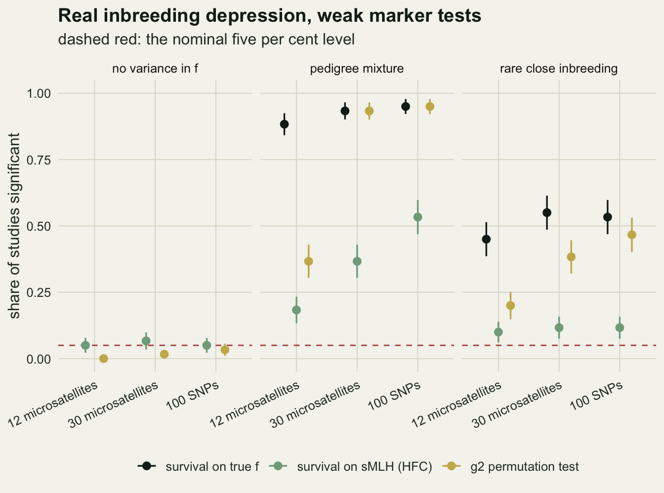
With no variance in f there is nothing to find. The HFC rejects in 0.05, 0.07 and 0.05 of studies for the three panels, at the nominal level within Monte Carlo error. The g2 test rejects in 0.00, 0.02 and 0.03, at or below the level; with 99 permutations the rule p < 0.05 has an exact size of 0.04 in any case, so the test is slightly conservative by construction.
Under the pedigree mixture, the regression on true f finds the effect in 0.88 of the studies in the 12 microsatellite cell (each panel has its own simulated studies, so this benchmark differs a little between panels by chance). The HFC on the same individuals and the same survival finds it in 0.18 with 12 microsatellites, 0.37 with 30 and 0.53 with 100 SNPs. The g2 test is significant in 0.37, 0.93 and 0.95 of studies. The g2 test falls short of the true f benchmark only for the small panel: at 30 microsatellites and 100 SNPs it is significant as often as the true f regression, while the HFC on the same studies finds the effect in about half of them at best. With rare close inbreeding everything is weaker, because a population with five per cent inbred individuals has little variance in f: the true f regression finds the effect in 0.45 of studies, the HFC in 0.10 at 12 microsatellites and 0.12 at 100 SNPs.
The closed forms are a check, not a finding
Two of the numbers above follow from arithmetic once g2 is known, and it is worth seeing them hold before trusting the rest. Because the markers affect survival only through f, the covariance of sMLH with survival is the covariance of their conditional means given f, and since expected sMLH is linear in f, the correlation factorises: r(sMLH, W) = r(sMLH, f) r(f, W). Szulkin and colleagues (2010) give this identity, and a second one that follows from the definition of g2: the squared correlation between heterozygosity and inbreeding is g2 divided by the variance of sMLH. Slate and colleagues (2004) made the same point earlier from the other side, that heterozygosity is a good proxy for inbreeding only when the variance in f is large.
cf <- summ[summ$scen != "no variance in f", ]
cf$r_hw_pred  <- cf$r_hf * cf$r_fw
cf$r2_hf_pred <- cf$g2 / cf$v_h
gap_rhw  <- max(abs(cf$r_hw - cf$r_hw_pred))
gap_r2   <- max(abs(cf$r2_hf - cf$r2_hf_pred))
m12_cf   <- cf[cf$panel == "12 microsatellites" & cf$scen == "pedigree mixture" &
               cf$n_ind == 200, ]
rel_12   <- m12_cf$r2_hf
Across the 12 cells with variance in f, the mean simulated r(sMLH, W) and the product of the mean r(sMLH, f) and mean r(f, W) differ by at most 0.011, and the mean squared correlation of sMLH with f differs from mean g2 over mean sMLH variance by at most 0.020. For the 12 microsatellite mixture cell, r(sMLH, f) is -0.38, r(f, W) is -0.22, and their product 0.085 sits beside a simulated r(sMLH, W) of 0.079.
Read as a measurement error problem, the squared correlation is the reliability of sMLH as a measure of f, here 0.15, and the correlation of heterozygosity with survival is the correlation of inbreeding with survival multiplied by its square root, 0.39. That is why the HFC is a small correlation even when inbreeding depression is severe.
cf$panel <- factor(cf$panel, levels = names(panels))
p_a <- ggplot(cf, aes(r_hw_pred, r_hw, colour = panel, shape = panel)) +
  geom_abline(slope = 1, intercept = 0, colour = te_body, linetype = "dashed") +
  geom_point(size = 2.4) +
  scale_colour_manual(values = c(te_sage, te_rust, te_ink), name = NULL) +
  scale_shape_manual(values = c(16, 17, 15), name = NULL) +
  labs(x = "r(sMLH, f) times r(f, W)", y = "simulated r(sMLH, W)",
       title = "Correlation with survival") +
  theme_datasheet()
p_b <- ggplot(cf, aes(r2_hf_pred, r2_hf, colour = panel, shape = panel)) +
  geom_abline(slope = 1, intercept = 0, colour = te_body, linetype = "dashed") +
  geom_point(size = 2.4) +
  scale_colour_manual(values = c(te_sage, te_rust, te_ink), name = NULL) +
  scale_shape_manual(values = c(16, 17, 15), name = NULL) +
  labs(x = "g2 / var(sMLH)", y = "simulated r(sMLH, f) squared",
       title = "Reliability of sMLH") +
  theme_datasheet()
(p_a | p_b) + plot_layout(guides = "collect") +
  plot_annotation(theme = theme_datasheet()) &
  theme(legend.position = "bottom")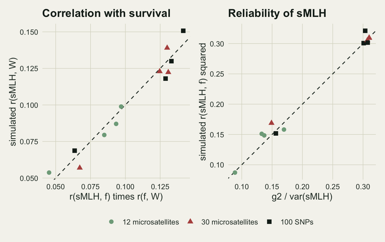
What the closed forms do not give is a test rate. Knowing that the expected correlation is small does not say how often a logistic regression on 200 individuals will reach p below 0.05, or how often a permutation test on a statistic of a few thousandths will. Those are what the grid measured, and what the rest of the post uses.
A non-significant g2 does not clear the panel
The usual advice is to report g2 alongside an HFC: if g2 is significant the panel captures variance in inbreeding and a general effect interpretation is available; if it is not, a significant HFC is more likely a local effect of a marker linked to a gene under selection. Szulkin and colleagues (2010) already warned that these quantities are imprecise when inbreeding is weak; the grid puts test rates on that warning. It also lets us ask what a non-significant g2 means when inbreeding depression is real by construction. A larger run of the 12 microsatellite mixture cell gives the joint rates enough precision.
n_joint <- 400
set.seed(1202)
joint_out <- t(replicate(n_joint, one_study(200, panels[[1]], scenarios[[2]])))
hfc_sig <- joint_out[, "p_hfc"] < 0.05
g2_sig  <- joint_out[, "p_g2"] < 0.05
share_g2_ns   <- mean(!g2_sig)
share_hfc_sig <- mean(hfc_sig)
hfc_given_g2  <- mean(hfc_sig[g2_sig])
hfc_given_ns  <- mean(hfc_sig[!g2_sig])
both_ns       <- mean(!hfc_sig & !g2_sig)
g2ns_among_hfc <- mean(!g2_sig[hfc_sig])
se_among_hfc  <- sqrt(g2ns_among_hfc * (1 - g2ns_among_hfc) / sum(hfc_sig))
se_both       <- sqrt(both_ns * (1 - both_ns) / n_joint)
se_joint <- sqrt(share_g2_ns * (1 - share_g2_ns) / n_joint)
se_hfc   <- sqrt(share_hfc_sig * (1 - share_hfc_sig) / n_joint)
se_given_g2 <- sqrt(hfc_given_g2 * (1 - hfc_given_g2) / sum(g2_sig))
se_given_ns <- sqrt(hfc_given_ns * (1 - hfc_given_ns) / sum(!g2_sig))
hfc_sig_g2_ns <- mean(hfc_sig & !g2_sig)
het_snp_mean <- mean(panels[[3]])

nax <- summ[summ$scen == "pedigree mixture", ]
m12_100 <- pick("12 microsatellites", n_ind = 100)
m12_400 <- pick("12 microsatellites", n_ind = 400)
s_100 <- pick("100 SNPs", n_ind = 100)
s_400 <- pick("100 SNPs", n_ind = 400)
In 400 studies of 200 individuals with 12 microsatellites and a strong, real general effect, the HFC is significant in 0.25 (Monte Carlo standard error 0.022) and g2 is not significant in 0.63 (standard error 0.024). Among the studies where g2 is significant, the HFC is significant in 0.26 (standard error 0.036); among those where g2 is not, in 0.24 (standard error 0.027). The g2 verdict carries little information about whether the HFC in the same study will be found. And among the studies with a significant HFC, 0.61 have a non-significant g2 on the same panel (standard error 0.049, out of 99 studies), about what independence of the two tests would give, since g2 is non-significant in 0.63 of all studies. Yet every one of those HFCs is a general effect of genome wide inbreeding and nothing else. In 0.48 of studies (standard error 0.025) both tests are negative, and the natural reading, that there is no inbreeding signal to find, is wrong.
Sample size moves both tests. A biallelic SNP carries less heterozygosity than a microsatellite (mean expected heterozygosity 0.38 for this SNP panel against 0.7), and in the figure 100 SNPs behave much like 30 microsatellites for g2, not like three times as many loci. The reliability of sMLH as a measure of f tells the same story: 0.32 for the SNP panel, 0.31 for 30 microsatellites and 0.15 for 12. With 12 microsatellites the g2 test rate goes from 0.27 at 100 individuals to 0.45 at 400, and the HFC from 0.12 to 0.45. With 100 SNPs the g2 rate goes from 0.73 to 1.00 and the HFC from 0.22 to 0.73.
n_long <- rbind(
  data.frame(panel = nax$panel, n_ind = nax$n_ind, rate = nax$hfc,
             test = "survival on sMLH (HFC)"),
  data.frame(panel = nax$panel, n_ind = nax$n_ind, rate = nax$g2sig,
             test = "g2 permutation test"),
  data.frame(panel = nax$panel, n_ind = nax$n_ind, rate = nax$truef,
             test = "survival on true f"))
n_long$panel <- factor(n_long$panel, levels = names(panels))
n_long$test <- factor(n_long$test, levels = c("survival on true f",
                      "survival on sMLH (HFC)", "g2 permutation test"))

ggplot(n_long, aes(n_ind, rate, colour = panel, shape = panel)) +
  geom_line(linewidth = 0.8) +
  geom_point(size = 2.2) +
  facet_wrap(~ test) +
  scale_x_continuous(breaks = c(100, 200, 400)) +
  scale_y_continuous(limits = c(0, 1)) +
  scale_colour_manual(values = c(te_sage, te_rust, te_ink), name = NULL) +
  scale_shape_manual(values = c(16, 17, 15), name = NULL) +
  labs(x = "individuals sampled", y = "share of studies significant",
       title = "Power grows with individuals, not only with loci",
       subtitle = "pedigree mixture, 70/20/10 per cent at f = 0, 0.125, 0.25") +
  theme_datasheet() +
  theme(legend.position = "bottom")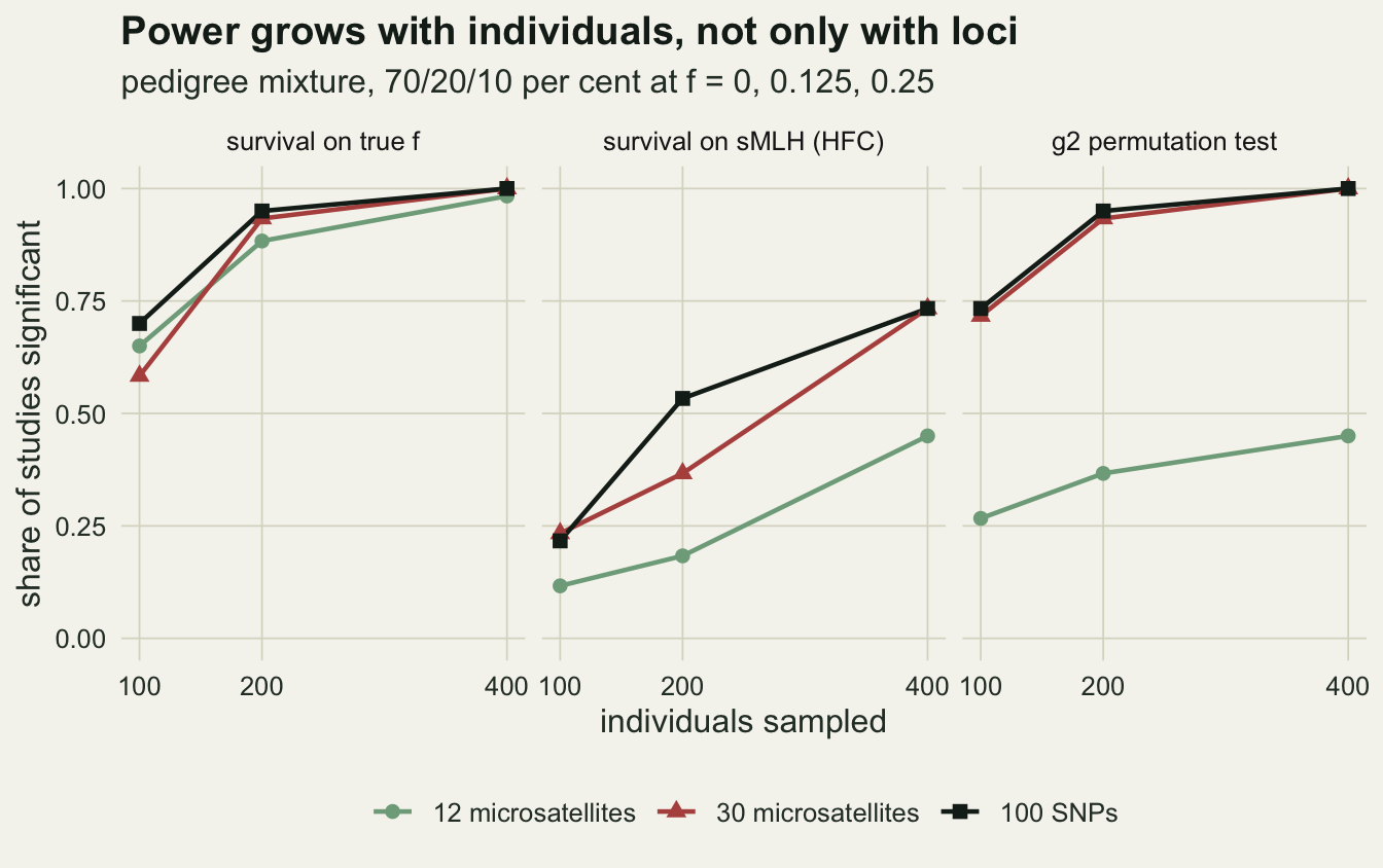
What to report
Report g2 with its confidence interval, not only its permutation p value. In the demonstration season above, 12 microsatellites gave an estimate of 0.0026 with a bootstrap interval from -0.0054 to 0.0127, which contains both zero and the population value 0.0076. The interval says how much variance in inbreeding the data could have hidden; the p value alone invites the reading that there was none.
Report the expected reliability of heterozygosity as a measure of inbreeding, g2 over the variance of sMLH, next to the HFC. Its square root is the factor by which the correlation of heterozygosity with fitness falls short of the correlation of inbreeding with fitness, and it turns a small HFC into a statement about the inbreeding effect it implies. Chapman and colleagues (2009) found HFCs in the published literature to be small on average, and a low reliability is the first explanation to check before reaching for a local effect.
Do not use a non-significant g2 as evidence that an HFC must be a local effect of a linked gene. In the simulation there are no local effects at all, and a non-significant g2 alongside a significant HFC happened in 0.15 of the 12 microsatellite studies. If the local versus general question matters, it needs more loci or more individuals, not a verdict from an underpowered test.
State the panel’s locus count, the heterozygosity per locus and the number of individuals together. The 100 SNP panel tested here gave sMLH about the same reliability as 30 microsatellites (0.32 against 0.31); its HFC rate of 0.53 against 0.37 differs by less than twice the Monte Carlo error of the difference, 0.090. Lower heterozygosity per locus is the likely reason more than three times as many loci did not do better, and it is invisible if only the locus count is reported.
Honest limits
Loci are unlinked and f is the pedigree coefficient, so every individual in a class has the same expected inbreeding. Real genomes are linked, and realised inbreeding varies around pedigree f through Mendelian sampling of chromosome segments. That variance adds to identity disequilibrium, and with dense SNP panels realised inbreeding can be measured much better than pedigree f. The simulation underestimates what a thousand SNPs can do, and that case was left out on purpose, both for knit time and because it needs a linkage model to be honest.
There are no local effects. A marker in linkage disequilibrium with a gene under selection gives an HFC that g2 is not designed to detect, and the post says nothing about how often that happens or how well the usual tests separate it from a general effect. The conclusion about non-significant g2 is only that it does not rule out the general case.
The fitness trait is binary survival with one strong inbreeding slope, and the tests use the whole sample in one logistic regression. Continuous traits, weaker inbreeding depression and additional covariates such as year or maternal identity all change power.
The inbreeding scenarios are three discrete pedigree mixtures. Populations with a long history of small size carry continuous variation in f from many ancestral loops, and the variance in f, not the mean, is what sets g2. The grid does not span the range of variance in f found in wild populations, and its rates should not be read across to a population whose variance in inbreeding is unknown.
Each cell has 60 studies, so every rate in the grid carries a Monte Carlo standard error of up to 0.065, and differences between neighbouring cells smaller than about twice that should not be ranked. The joint rates for the 12 microsatellite cell use 400 studies for that reason.
References
Chapman JR, Nakagawa S, Coltman DW, Slate J, Sheldon BC 2009 Molecular Ecology 18(13):2746-2765 (10.1111/j.1365-294X.2009.04247.x)
David P, Pujol B, Viard F, Castella V, Goudet J 2007 Molecular Ecology 16(12):2474-2487 (10.1111/j.1365-294X.2007.03330.x)
Stoffel MA, Esser M, Kardos M, Humble E, Nichols H, David P, Hoffman JI 2016 Methods in Ecology and Evolution 7(11):1331-1339 (10.1111/2041-210X.12588)
Coltman DW, Pilkington JG, Smith JA, Pemberton JM 1999 Evolution 53(4):1259-1267 (10.1111/j.1558-5646.1999.tb04538.x)
Slate J, David P, Dodds KG, Veenvliet BA, Glass BC, Broad TE, McEwan JC 2004 Heredity 93(3):255-265 (10.1038/sj.hdy.6800485)
Szulkin M, Bierne N, David P 2010 Evolution 64(5):1202-1217 (10.1111/j.1558-5646.2010.00966.x)