library(ggplot2)
library(patchwork)

te_paper  <- "#f5f4ee"
te_ink    <- "#16241d"
te_body   <- "#2c3a31"
te_forest <- "#275139"
te_rust   <- "#b5534e"
te_gold   <- "#c9b458"
te_line   <- "#dad9ca"

theme_datasheet <- function() {
  theme_minimal(base_size = 12) +
    theme(plot.background  = element_rect(fill = te_paper, colour = NA),
          panel.background = element_rect(fill = te_paper, colour = NA),
          panel.grid.major = element_line(colour = te_line, linewidth = 0.3),
          panel.grid.minor = element_blank(),
          text             = element_text(colour = te_body),
          plot.title       = element_text(colour = te_ink, face = "bold"),
          plot.subtitle    = element_text(colour = te_body),
          axis.text        = element_text(colour = te_body),
          strip.text       = element_text(colour = te_ink, face = "bold"))
}Extra-pair paternity from parentage mismatches
R
population genetics
parentage
genotyping error
simulation
ecology tutorial
A fixed mismatch rule turns genotyping error into extra-pair paternity as loci are added. Measuring in R the brother problem and two repairs that fit the rate.
A field team has ringed the chicks of a nest box population of blue tits for three seasons, taken a blood drop from every chick and both attending adults, and sent the samples off for a panel of microsatellites. The spreadsheet that comes back has one row per chick. The mother is almost never in doubt, because she was caught on the nest. The question is the father, and the rule most studies use is plain: if the chick carries an allele at some locus that neither the mother nor the social male could have given it, that locus is a mismatch, and a chick with at least one mismatch (or at least two, in the more careful papers) is scored as extra-pair. The proportion of such chicks is the extra-pair paternity rate, and it is the number that goes into the abstract.
The post on checking an animal model takes that number as an input. Its first check corrupts a known fraction of sire links and measures what the wrong fathers do to heritability, and it ends with the practical advice that the check for pedigree error is molecular: genotype a sample of broods and estimate the extra-pair rate. This post picks up from that sentence and asks where the rate comes from. The answer is that a good part of it can be a property of the marker panel and the exclusion rule rather than of the birds.
Two other posts here touch the same data without asking this question. Checking a population genetics analysis treats allelic dropout as a marker artefact that inflates Fis at a few loci, a problem of population summaries rather than of individual fathers. Assignment tests and self-assignment has an exclusion test, but it excludes an individual from a source population, with no genotyping error in the model. Parentage exclusion is the same logic applied to one trio at a time, and genotyping error is what breaks it.
The post does four things. It writes the false exclusion rate of a fixed mismatch rule in closed form and checks it against simulation, because that part is arithmetic and should be treated as such. It measures what happens when the extra-pair sire is a brother of the social male, which no closed form here covers. It fits a two-component mixture to the mismatch counts and reads the rate off the fit, with no threshold. Finally it builds an error-aware likelihood ratio, calibrates its threshold by simulation, and tests both repairs on a study-sized sample under assumptions that are wrong in two different ways.
Trios, mismatches and an error model
Each simulated brood is a trio: a mother, a social male and one chick. With probability one tenth the chick was sired by another male. A genotype is a pair of allele calls per locus, and the error model is the simplest one in use: each allele call in the chick, the mother and the social male is independently replaced, with probability e, by an allele drawn from the population frequencies. The replacement can return the true allele, so the rate at which a call actually changes is a little below e. A locus is a mismatch when no assignment of the chick’s two alleles puts one in the mother and the other in the social male.
Microsatellite loci carry eight alleles each, with frequencies drawn from a symmetric Dirichlet distribution with shape 0.8. That gives the uneven spectrum real microsatellites have: one or two common alleles and a tail of rare ones. The panels are nested, so the 8 locus panel is the first 8 loci of the 15 locus panel and so on, which keeps comparisons between panel sizes free of a fresh frequency draw.
n_allele  <- 8
dir_shape <- 0.8

draw_freqs <- function(n_loc, n_al, shape) {
  lapply(seq_len(n_loc), function(i) { x <- rgamma(n_al, shape); x / sum(x) })
}
draw_geno <- function(n, fr) {
  geno <- array(0L, c(n, 2, length(fr)))
  for (l in seq_along(fr)) {
    geno[, , l] <- sample.int(length(fr[[l]]), 2 * n, TRUE, fr[[l]])
  }
  geno
}
add_error <- function(geno, e_rate, fr) {
  if (e_rate == 0) return(geno)
  for (l in seq_along(fr)) {
    hit <- runif(2 * dim(geno)[1]) < e_rate
    if (any(hit)) {
      calls <- geno[, , l]
      calls[hit] <- sample.int(length(fr[[l]]), sum(hit), TRUE, fr[[l]])
      geno[, , l] <- calls
    }
  }
  geno
}
transmit <- function(parent) {
  n <- dim(parent)[1]; n_loc <- dim(parent)[3]
  pick <- sample.int(2, n * n_loc, TRUE)
  matrix(parent[cbind(rep(seq_len(n), n_loc), pick,
                      rep(seq_len(n_loc), each = n))], n, n_loc)
}
make_chick <- function(mum, dad) {
  chick <- array(0L, dim(mum))
  chick[, 1, ] <- transmit(mum)
  chick[, 2, ] <- transmit(dad)
  chick
}
locus_mismatch <- function(chick, mum, soc) {
  a1 <- chick[, 1, ]; a2 <- chick[, 2, ]
  in_mum <- function(a) a == mum[, 1, ] | a == mum[, 2, ]
  in_soc <- function(a) a == soc[, 1, ] | a == soc[, 2, ]
  !((in_mum(a1) & in_soc(a2)) | (in_mum(a2) & in_soc(a1)))
}
nested_counts <- function(mis, panels) {
  cum <- t(apply(mis, 1, cumsum))
  cum[, panels, drop = FALSE]
}
brood_set <- function(n, fr, e_rate, epp, sire) {
  mum <- draw_geno(n, fr)
  if (sire == "unrelated") {
    soc <- draw_geno(n, fr); other <- draw_geno(n, fr)
  } else {
    gran_f <- draw_geno(n, fr); gran_m <- draw_geno(n, fr)
    soc <- make_chick(gran_f, gran_m); other <- make_chick(gran_f, gran_m)
  }
  is_ep <- runif(n) < epp
  sire_g <- soc
  sire_g[is_ep, , ] <- other[is_ep, , ]
  chick <- make_chick(mum, sire_g)
  list(chick = add_error(chick, e_rate, fr), mum = add_error(mum, e_rate, fr),
       soc = add_error(soc, e_rate, fr), is_ep = is_ep)
}
A fixed rule is binomial arithmetic
Before simulating anything, the rate a fixed rule reports can be written down. At one locus let w be the probability that a within-pair chick shows a mismatch (only error can cause one) and x the probability that an extra-pair chick shows one. Loci are independent, so the mismatch count is a sum of independent Bernoulli variables, and the probability of at least k mismatches is a tail of that Poisson binomial distribution. The reported rate under a k mismatch rule is then the true rate times the tail for extra-pair chicks plus the within-pair share times the tail for within-pair chicks, which is the false exclusion rate.
The per-locus probabilities are exact too. The error model is a transition matrix from true to observed allele, and summing over true genotypes and transmissions gives the joint distribution of the observed parental genotype and the observed allele it passed on. Pairing the mother’s table with the social male’s table (or with a random male’s, for an extra-pair chick) and adding up the inconsistent combinations gives w and x with no simulation.
exact_locus <- function(f, e_rate) {
  k <- length(f)
  tr_mat <- (1 - e_rate) * diag(k) + e_rate * matrix(f, k, k, byrow = TRUE)
  q_mat  <- t(tr_mat) %*% (f * tr_mat)
  cells  <- expand.grid(h1 = 1:k, h2 = 1:k, o = 1:k)
  p_par  <- 0.5 * (q_mat[cbind(cells$h1, cells$o)] * f[cells$h2] +
                   f[cells$h1] * q_mat[cbind(cells$h2, cells$o)])
  p_rand <- f[cells$h1] * f[cells$h2] * f[cells$o]
  n_cell <- nrow(cells)
  i_m <- rep(seq_len(n_cell), times = n_cell)
  i_s <- rep(seq_len(n_cell), each = n_cell)
  o1 <- cells$o[i_m]; o2 <- cells$o[i_s]
  in_m <- function(a) a == cells$h1[i_m] | a == cells$h2[i_m]
  in_s <- function(a) a == cells$h1[i_s] | a == cells$h2[i_s]
  bad <- !((in_m(o1) & in_s(o2)) | (in_m(o2) & in_s(o1)))
  c(within = sum(p_par[i_m] * p_par[i_s] * bad),
    extra  = sum(p_par[i_m] * p_rand[i_s] * bad))
}
tail_prob <- function(p_loc, k_rule) {
  pmf <- 1
  for (q in p_loc) pmf <- c(pmf * (1 - q), 0) + c(0, pmf * q)
  sum(pmf[(k_rule + 1):length(pmf)])
}

set.seed(3107)
max_loc  <- 25
fr_ms    <- draw_freqs(max_loc, n_allele, dir_shape)
panel_ms <- c(8, 15, 25)
err_grid <- c(0, 0.005, 0.01, 0.02)
epp_true <- 0.10

exact_tab <- do.call(rbind, lapply(err_grid, function(e_rate) {
  p_loc <- t(vapply(fr_ms, exact_locus, numeric(2), e_rate = e_rate))
  do.call(rbind, lapply(panel_ms, function(n_loc) {
    do.call(rbind, lapply(1:2, function(k_rule) {
      fe <- tail_prob(p_loc[1:n_loc, "within"], k_rule)
      ce <- tail_prob(p_loc[1:n_loc, "extra"], k_rule)
      data.frame(e_rate = e_rate, n_loc = n_loc, k_rule = k_rule,
                 false_ex = fe, catch = ce,
                 rate = epp_true * ce + (1 - epp_true) * fe,
                 p_within = mean(p_loc[1:n_loc, "within"]))
    }))
  }))
}))
pick_ex <- function(e_rate, n_loc, k_rule, col) {
  exact_tab[exact_tab$e_rate == e_rate & exact_tab$n_loc == n_loc &
              exact_tab$k_rule == k_rule, col]
}
w_one   <- pick_ex(0.01, 25, 1, "p_within")
c_fac   <- w_one / 0.01
w_loc_fac <- vapply(fr_ms, function(f) exact_locus(f, 0.01)[["within"]], numeric(1)) / 0.01
c_even  <- exact_locus(rep(1 / n_allele, n_allele), 0.01)[["within"]] / 0.01
approx8 <- 1 - (1 - w_one)^8
approx25 <- 1 - (1 - w_one)^25
At an allele error rate of 0.01, the per-locus mismatch probability for a within-pair chick averages 0.0219 over the 25 loci, which is 2.19 times the error rate: six allele calls go into a trio, and only some replacements create an inconsistency. The multiplier is not a constant: it depends on the allele frequencies, running from 1.24 to 2.69 across these 25 loci and reaching 2.94 for a locus with 8 equally common alleles. The one-line approximation 1 - (1 - w)^L then gives a false exclusion rate of 0.163 at 8 loci and 0.426 at 25, against exact values of 0.162 and 0.426.
With a true rate of 0.10, the one mismatch rule reports 0.246, 0.351 and 0.483 at 8, 15 and 25 loci. The two mismatch rule reports 0.109, 0.136 and 0.193. Adding loci, usually presented as an improvement, raises the reported rate under both rules, because extra-pair chicks are already caught on small panels (the two mismatch rule catches 0.984 of unrelated extra-pair chicks at 8 loci) while every added locus is another chance for error. At an error rate of 0.02 and 25 loci the one mismatch rule reports 0.703.
n_brood <- 4000
set.seed(3108)
sim_tab <- do.call(rbind, lapply(err_grid, function(e_rate) {
  bs  <- brood_set(n_brood, fr_ms, e_rate, epp_true, "unrelated")
  cnt <- nested_counts(locus_mismatch(bs$chick, bs$mum, bs$soc), panel_ms)
  do.call(rbind, lapply(1:2, function(k_rule) {
    data.frame(e_rate = e_rate, n_loc = panel_ms, k_rule = k_rule,
               sim_rate = colMeans(cnt >= k_rule))
  }))
}))
check_tab <- merge(exact_tab, sim_tab)
check_tab$z <- (check_tab$sim_rate - check_tab$rate) /
  sqrt(check_tab$rate * (1 - check_tab$rate) / n_brood)
max_z <- max(abs(check_tab$z))
The simulation agrees. Across all 24 combinations of error rate, panel and rule, 4000 simulated broods per error rate put the reported rate within 1.55 binomial standard errors of the closed form. The standard errors are computed as if the cells were independent, which they are not (the three panels share broods), so the check is a sanity check, not a test. Nothing in this section needed a simulation to be known; the rest of the post does.
plot_ex <- exact_tab
plot_ex$rule <- ifelse(plot_ex$k_rule == 1, "one mismatch excludes", "two mismatches exclude")
plot_sim <- check_tab
plot_sim$rule <- ifelse(plot_sim$k_rule == 1, "one mismatch excludes", "two mismatches exclude")
plot_ex$err  <- factor(plot_ex$e_rate)
plot_sim$err <- factor(plot_sim$e_rate)
ggplot(plot_ex, aes(n_loc, rate, colour = err)) +
  geom_line(linewidth = 0.9) +
  geom_point(data = plot_sim, aes(y = sim_rate), size = 2.2, shape = 21,
             fill = te_paper, stroke = 1) +
  facet_wrap(~ rule) +
  scale_colour_manual(values = c(te_ink, te_forest, te_gold, te_rust),
                      name = "allele error rate") +
  scale_x_continuous(breaks = panel_ms) +
  labs(x = "microsatellite loci", y = "reported extra-pair rate",
       title = "More loci, more extra-pair paternity",
       subtitle = "the zero error line sits on the true rate, 0.10") +
  theme_datasheet() +
  theme(legend.position = "bottom")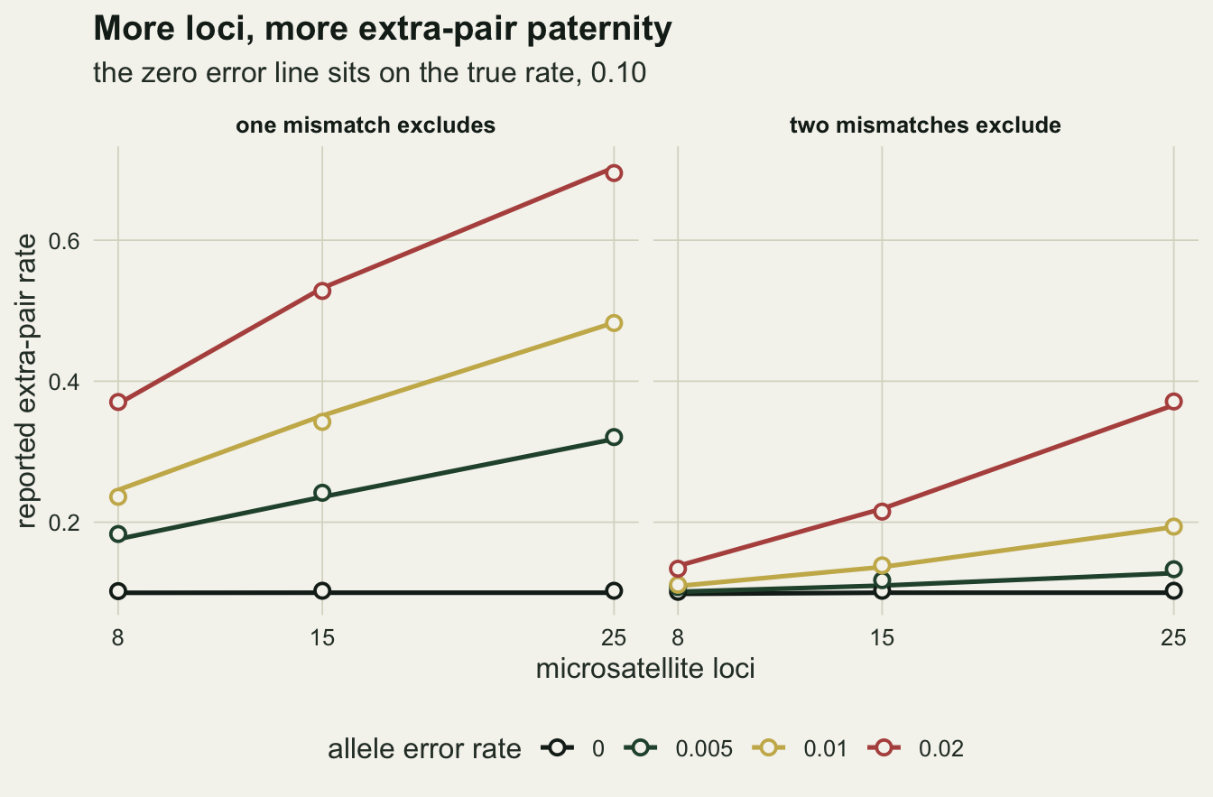
A brother of the social male
Error pushes the reported rate up. Relatedness between the social male and the true sire pushes it down, because a brother shares half his alleles with the male whose paternity is being tested and his chicks fail to mismatch far more often than a stranger’s. Brothers are not an exotic case in birds with natal philopatry, and neighbouring territory holders are often kin. There is no closed form in this post for the brother case, so it is simulated: every chick below is extra-pair, sired by a full brother of the social male, and the quantity measured is the fraction that escapes exclusion.
The brother result depends on the allele frequency spectrum as much as on the number of loci, so it is run twice: on the skewed Dirichlet frequencies used above and on an even spectrum where all eight alleles have frequency one eighth. The even spectrum is the most informative a locus with eight alleles can be, and no real microsatellite panel reaches it.
fr_even <- replicate(max_loc, rep(1 / n_allele, n_allele), simplify = FALSE)
spectra <- list(skewed = fr_ms, even = fr_even)
het_of  <- function(fr) mean(vapply(fr, function(f) 1 - sum(f^2), numeric(1)))
neff_of <- function(fr) mean(vapply(fr, function(f) 1 / sum(f^2), numeric(1)))
excl_of <- function(fr) mean(vapply(fr, function(f) exact_locus(f, 0)[["extra"]], numeric(1)))
spec_tab <- data.frame(spectrum = names(spectra),
                       he   = vapply(spectra, function(fr) het_of(fr[1:8]), numeric(1)),
                       n_eff = vapply(spectra, function(fr) neff_of(fr[1:8]), numeric(1)),
                       excl = vapply(spectra, function(fr) excl_of(fr[1:8]), numeric(1)))

set.seed(3109)
bro_tab <- do.call(rbind, lapply(names(spectra), function(sp) {
  do.call(rbind, lapply(c(0, 0.01), function(e_rate) {
    do.call(rbind, lapply(c("brother", "unrelated"), function(sire) {
      bs  <- brood_set(n_brood, spectra[[sp]], e_rate, 1, sire)
      cnt <- nested_counts(locus_mismatch(bs$chick, bs$mum, bs$soc), panel_ms)
      data.frame(spectrum = sp, e_rate = e_rate, sire = sire, n_loc = panel_ms,
                 miss1 = colMeans(cnt < 1), miss2 = colMeans(cnt < 2),
                 med = apply(cnt, 2, median))
    }))
  }))
}))
pick_bro <- function(sp, e_rate, sire, n_loc, col) {
  bro_tab[bro_tab$spectrum == sp & bro_tab$e_rate == e_rate &
            bro_tab$sire == sire & bro_tab$n_loc == n_loc, col]
}
The first 8 skewed loci have a mean expected heterozygosity of 0.749, an effective number of alleles of 4.19, and a single locus mismatches an unrelated extra-pair chick with probability 0.553 in the absence of error. The even spectrum has 0.875, 8.00 and 0.743. Those are the three numbers to quote with any brother result.
With no genotyping error at all, the two mismatch rule lets 0.305 of brother-sired chicks through at 8 skewed loci, and the one mismatch rule lets through 0.073. On the even spectrum the same two numbers are 0.135 and 0.026: less than half the skewed values, from the same number of loci. The median mismatch count of a brother-sired chick at 8 skewed loci is 2, against 4 for an unrelated sire. At 15 skewed loci the two mismatch rule misses 0.056 of brother-sired chicks, and at 25 loci 0.0057.
This is where no fixed threshold works on a small panel. On 8 skewed loci with an allele error rate of 0.01, the one mismatch rule falsely excludes 0.162 of within-pair chicks; moving to two mismatches cuts that to 0.012 but lets 0.279 of brother-sired chicks through. One rule is wrong about the social male’s own chicks and the other is wrong about his brother’s. On 25 loci the brother problem has gone and the error problem has grown, so the rule that suits one panel is the wrong rule for the other.
bro_plot <- bro_tab[bro_tab$e_rate == 0 & bro_tab$sire == "brother", ]
bro_long <- rbind(
  data.frame(bro_plot[, c("spectrum", "n_loc")], miss = bro_plot$miss1,
             rule = "one mismatch excludes"),
  data.frame(bro_plot[, c("spectrum", "n_loc")], miss = bro_plot$miss2,
             rule = "two mismatches exclude"))
bro_long$spectrum <- ifelse(bro_long$spectrum == "skewed",
                            "skewed frequencies (Dirichlet 0.8)", "even frequencies")
ggplot(bro_long, aes(n_loc, miss, colour = spectrum)) +
  geom_line(linewidth = 0.9) +
  geom_point(size = 2.4) +
  facet_wrap(~ rule) +
  scale_colour_manual(values = c(te_gold, te_forest), name = NULL) +
  scale_x_continuous(breaks = panel_ms) +
  labs(x = "microsatellite loci", y = "brother-sired chicks not excluded",
       title = "A brother escapes a small panel",
       subtitle = "every chick here is extra-pair; no genotyping error") +
  theme_datasheet() +
  theme(legend.position = "bottom")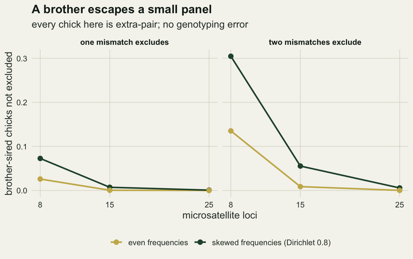
Reading the rate from the mismatch distribution
A threshold throws away the shape of the mismatch counts. Plotted as a histogram, the counts of a sample of chicks form two humps: within-pair chicks pile up at zero or one, with a tail set by the error rate, and extra-pair chicks sit further out, at a distance set by the panel and by how related the true sire is. Fitting a two-component mixture to that histogram estimates the extra-pair share directly, as the weight of the outer component, and it needs neither a threshold nor a value for the error rate.
The mixture used here is the plainest one: each component is binomial in the number of loci with its own per-locus mismatch probability, fitted by EM in the way the post on fitting a mixture of normals fits normal components. The binomial is a slight misfit, because per-locus probabilities differ between loci and the true count is Poisson binomial, which is slightly less variable than a binomial with the same mean. The panels now include biallelic SNPs, 60, 120 and 240 of them, with minor allele frequencies drawn uniformly between 0.2 and 0.5.
snp_loc   <- 240
panel_snp <- c(60, 120, 240)
set.seed(3110)
fr_snp <- lapply(runif(snp_loc, 0.2, 0.5), function(q) c(q, 1 - q))
c_snp  <- mean(vapply(fr_snp[1:60], function(f) exact_locus(f, 0.01)[["within"]], numeric(1))) / 0.01

em_binmix <- function(x, n_loc, iter = 150) {
  pi_ep <- 0.2; p_wp <- 0.01; p_ep <- 0.2
  for (i in seq_len(iter)) {
    d_ep <- pi_ep * dbinom(x, n_loc, p_ep)
    d_wp <- (1 - pi_ep) * dbinom(x, n_loc, p_wp)
    w_ep <- d_ep / (d_ep + d_wp)
    pi_ep <- mean(w_ep)
    p_ep  <- sum(w_ep * x) / (n_loc * max(sum(w_ep), 1e-9))
    p_wp  <- sum((1 - w_ep) * x) / (n_loc * sum(1 - w_ep))
  }
  c(pi_ep = pi_ep, p_wp = p_wp, p_ep = p_ep)
}

e_mix <- 0.01
mix_runs <- list()
mix_tab <- do.call(rbind, lapply(c("unrelated", "brother"), function(sire) {
  do.call(rbind, lapply(c("microsatellite", "SNP"), function(kind) {
    fr   <- if (kind == "SNP") fr_snp else fr_ms
    pans <- if (kind == "SNP") panel_snp else panel_ms
    bs  <- brood_set(n_brood, fr, e_mix, epp_true, sire)
    cnt <- nested_counts(locus_mismatch(bs$chick, bs$mum, bs$soc), pans)
    mix_runs[[paste(sire, kind)]] <<- list(cnt = cnt, is_ep = bs$is_ep)
    do.call(rbind, lapply(seq_along(pans), function(j) {
      x <- cnt[, j]; fit <- em_binmix(x, pans[j])
      data.frame(sire = sire, kind = kind, n_loc = pans[j], true = mean(bs$is_ep),
                 rule1 = mean(x >= 1), rule2 = mean(x >= 2),
                 ep_med = median(x[bs$is_ep]),
                 wp_q99 = unname(quantile(x[!bs$is_ep], 0.99, type = 1)),
                 em = fit[["pi_ep"]], p_wp = fit[["p_wp"]], p_ep = fit[["p_ep"]])
    }))
  }))
}))
pick_mix <- function(sire, n_loc, col) {
  mix_tab[mix_tab$sire == sire & mix_tab$n_loc == n_loc, col]
}
mix_gap <- max(abs(mix_tab$em - mix_tab$true))
The per-locus within-pair mismatch probability on the first 60 of these SNPs is only 0.68 times the error rate, against 2.19 on the microsatellites, because a replacement drawn from two alleles often returns the allele that was already there. With unrelated extra-pair sires and an allele error rate of 0.01, the median extra-pair chick shows 10, 20 and 41 mismatches on 60, 120 and 240 SNPs, while 99 per cent of within-pair chicks show at most 2, 4 and 5. The humps separate cleanly, and the fixed rules do worst exactly here, because a SNP mismatches an extra-pair chick rarely and error has many loci to act on: the one mismatch rule reports 0.821 at 240 SNPs and the two mismatch rule 0.535, from a realised rate of 0.102.
The mixture weight on the same counts is 0.102. Over all 12 panels in the table, unrelated and brother sires, microsatellites and SNPs, the largest gap between the mixture estimate and the realised rate in these samples of 4000 chicks is 0.014, and it is in the hardest cell: 8 microsatellites with brother sires, where the mixture gives 0.091 from a realised 0.104. With brother sires the outer hump moves in to a median of 5 mismatches at 60 SNPs and 2 at 8 microsatellites, and the figure below shows the humps touching at 60 SNPs and running into each other at 8 microsatellites. Four thousand chicks is far more than a study has, so the small-sample behaviour is left for the next section.
hist_panel <- function(key, j, n_loc, lab, y_lab = NULL) {
  run <- mix_runs[[key]]
  x   <- run$cnt[, j]
  fit <- em_binmix(x, n_loc)
  x_max <- max(x)
  obs <- rbind(
    data.frame(k = 0:x_max, n = tabulate(x[!run$is_ep] + 1, x_max + 1), who = "within-pair"),
    data.frame(k = 0:x_max, n = tabulate(x[run$is_ep] + 1, x_max + 1), who = "extra-pair"))
  fitted <- data.frame(k = 0:x_max,
                       n = length(x) * (fit[["pi_ep"]] * dbinom(0:x_max, n_loc, fit[["p_ep"]]) +
                                        (1 - fit[["pi_ep"]]) * dbinom(0:x_max, n_loc, fit[["p_wp"]])))
  obs$who <- factor(obs$who, levels = c("within-pair", "extra-pair"))
  n_wp <- obs$n[obs$who == "within-pair"]
  obs$ymin <- ifelse(obs$who == "within-pair", 0, n_wp)
  obs$ymax <- obs$ymin + obs$n
  ggplot(obs) +
    geom_rect(aes(xmin = k - 0.45, xmax = k + 0.45, ymin = ymin, ymax = ymax, fill = who)) +
    geom_point(data = fitted, aes(k, n), colour = te_ink, size = 1.3) +
    scale_fill_manual(values = c("extra-pair" = te_rust, "within-pair" = te_line), name = NULL) +
    scale_y_sqrt() +
    labs(x = "mismatching loci", y = y_lab, title = lab) +
    theme_datasheet() +
    theme(plot.title = element_text(size = 11))
}
hist_panel("brother microsatellite", 1, 8, "8 loci, brother sires",
           "chicks (square root scale)") +
  hist_panel("brother SNP", 1, 60, "60 SNPs, brother sires") +
  hist_panel("unrelated SNP", 2, 120, "120 SNPs, unrelated") +
  plot_layout(guides = "collect") +
  plot_annotation(title = "Two humps, and where they meet",
                  subtitle = "black points: expected counts under the fitted mixture",
                  theme = theme_datasheet()) &
  theme(legend.position = "bottom")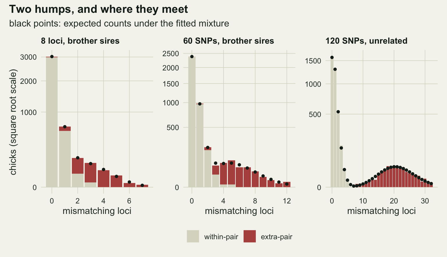
An error-aware likelihood ratio, calibrated by simulation
The route most parentage software takes is a likelihood ratio. For each chick, compare the probability of its genotype given the mother and the social male with the probability given the mother and a random male from the population, and add the logarithms over loci. A zero likelihood from one mismatching locus would sink the social male outright, so an error term is mixed in: with probability eps the chick’s genotype is treated as a random draw from Hardy-Weinberg proportions. Marshall et al. 1998 introduced this form and Kalinowski et al. 2007 revised how the error term enters; the version here puts the error term on the chick only and assumes the parental genotypes are right. That is close to the original Marshall et al. 1998 form and omits the Kalinowski et al. 2007 correction, and the threshold here is set on the social male’s log ratio directly rather than on the difference between the top two candidates that CERVUS uses.
A threshold on the log ratio still has to be chosen, and it is chosen by simulation. Twenty thousand within-pair and twenty thousand extra-pair chicks are simulated under the assumed error rate of 0.01 with unrelated extra-pair sires; the threshold is set so that 1 per cent of within-pair chicks fall below it, and the simulated fraction of extra-pair chicks that stay above it is recorded. The true sire is never among the candidates, here or in the calibration, because the alternative hypothesis is a random male rather than a named one. The observed fraction below the threshold, q_obs, is then corrected with the two calibration rates a (false exclusion) and b (miss) as (q_obs - a) / (1 - a - b), the standard correction for a classifier with known error rates.
lod_social <- function(chick, mum, soc, fr, eps) {
  lod <- numeric(dim(chick)[1])
  for (l in seq_along(fr)) {
    f <- fr[[l]]
    o1 <- chick[, 1, l]; o2 <- chick[, 2, l]
    m1 <- mum[, 1, l]; m2 <- mum[, 2, l]; s1 <- soc[, 1, l]; s2 <- soc[, 2, l]
    hom  <- o1 == o2
    p_hw <- ifelse(hom, f[o1]^2, 2 * f[o1] * f[o2])
    gives <- function(a, b) ifelse(hom, (a == o1) * (b == o1),
                                   (a == o1) * (b == o2) + (a == o2) * (b == o1))
    t_soc <- 0.25 * (gives(m1, s1) + gives(m1, s2) + gives(m2, s1) + gives(m2, s2))
    from_m1 <- 0.5 * ((m1 == o1) + (m2 == o1))
    from_m2 <- 0.5 * ((m1 == o2) + (m2 == o2))
    t_rand <- ifelse(hom, from_m1 * f[o1], from_m1 * f[o2] + from_m2 * f[o1])
    lod <- lod + log((1 - eps) * t_soc + eps * p_hw) -
      log((1 - eps) * t_rand + eps * p_hw)
  }
  lod
}

eps_assumed <- 0.02
e_assumed   <- 0.01
n_cal       <- 20000
alpha_cal   <- 0.01
set.seed(3111)
cal_tab <- as.data.frame(do.call(rbind, lapply(panel_ms[1:2], function(n_loc) {
  fr <- fr_ms[1:n_loc]
  wp <- brood_set(n_cal, fr, e_assumed, 0, "unrelated")
  ep <- brood_set(n_cal, fr, e_assumed, 1, "unrelated")
  lod_wp <- lod_social(wp$chick, wp$mum, wp$soc, fr, eps_assumed)
  lod_ep <- lod_social(ep$chick, ep$mum, ep$soc, fr, eps_assumed)
  thr <- unname(quantile(lod_wp, alpha_cal))
  c(n_loc = n_loc, thr = thr, false_ex = mean(lod_wp < thr),
    miss = mean(lod_ep >= thr))
})))
The genotype-level error weight eps is set to 0.02, twice the allele error rate, because a genotype has two allele calls. On 8 loci the calibrated threshold is a log ratio of -0.81, and it misses 0.0103 of unrelated extra-pair chicks; on 15 loci the threshold is 3.68 and the miss rate is 0.0001. Both false exclusion rates are 0.01 by construction.
The test is a study of realistic size: 200 chicks with a true extra-pair probability of 0.10, repeated 300 times in each of three situations. In the first the calibration assumptions hold. In the second the real allele error rate is twice the assumed one, which is the ordinary state of a new microsatellite panel before anyone has regenotyped a sample. In the third the error rate is right but every extra-pair sire is a brother of the social male. The mixture and the plain two mismatch rule are scored on the same chicks.
n_study <- 200
n_rep   <- 300
scen <- data.frame(label = c("as assumed", "error doubled", "brother sires"),
                   e_rate = c(e_assumed, 2 * e_assumed, e_assumed),
                   sire = c("unrelated", "unrelated", "brother"))
method_lab <- c("likelihood ratio, corrected", "mixture", "two mismatch rule")
set.seed(3112)
study_tab <- do.call(rbind, lapply(seq_len(nrow(cal_tab)), function(j) {
  n_loc <- cal_tab$n_loc[j]; fr <- fr_ms[1:n_loc]
  do.call(rbind, lapply(seq_len(nrow(scen)), function(s) {
    est <- replicate(n_rep, {
      bs  <- brood_set(n_study, fr, scen$e_rate[s], epp_true, scen$sire[s])
      lod <- lod_social(bs$chick, bs$mum, bs$soc, fr, eps_assumed)
      cnt <- rowSums(locus_mismatch(bs$chick, bs$mum, bs$soc))
      raw <- mean(lod < cal_tab$thr[j])
      c(truth = mean(bs$is_ep),
        lr = (raw - cal_tab$false_ex[j]) / (1 - cal_tab$false_ex[j] - cal_tab$miss[j]),
        mix = em_binmix(cnt, n_loc)[["pi_ep"]],
        rule2 = mean(cnt >= 2))
    })
    err <- est[c("lr", "mix", "rule2"), ] - rep(est["truth", ], each = 3)
    data.frame(n_loc = n_loc, scenario = scen$label[s], method = method_lab,
               bias = rowMeans(err), sd_err = apply(err, 1, sd),
               mc_se = apply(err, 1, sd) / sqrt(n_rep))
  }))
}))
pick_st <- function(n_loc, scenario, method, col) {
  study_tab[study_tab$n_loc == n_loc & study_tab$scenario == scenario &
              study_tab$method == method, col]
}
lr_lab <- method_lab[1]; mx_lab <- method_lab[2]; r2_lab <- method_lab[3]
max_mcse <- max(study_tab$mc_se)
Errors below are estimate minus the realised rate in each sample, and the largest Monte Carlo standard error of any mean error is 0.0033. When the assumptions hold, the corrected likelihood ratio is nearly unbiased on both panels: mean error -0.0013 on 8 loci and 0.0005 on 15, with a standard deviation of 0.0068 on 15 loci. The mixture on 15 loci has a mean error of 0.0001 and a standard deviation of 0.0023, smaller than the likelihood ratio’s: on 15 loci the humps barely overlap, so the fitted weight tracks the realised number of extra-pair chicks, while the likelihood ratio subtracts an expected number of false exclusions from a count that varies around it. The two mismatch rule is off by 0.0369 on 15 loci before anything has gone wrong.
When the real error rate is twice the assumed one, the calibration is out of date and the corrected likelihood ratio overestimates by 0.0136 on 8 loci and 0.0254 on 15; the true rate is 0.10, so on 15 loci that is a quarter of it. The mixture, which was never told the error rate, stays at 0.0028 and 0.0006. The two mismatch rule reaches 0.118 on 15 loci.
Brother sires break both repairs on the small panel. The corrected likelihood ratio underestimates by 0.0326 on 8 loci, because its miss rate was calibrated on strangers. The mixture is worse in a different way: its mean error is 0.0189, but its standard deviation is 0.0564, more than half the true rate, because with 200 chicks and humps that overlap, the fitted weight swings widely from one sample to the next. The two mismatch rule lands at -0.0173 in the same cell, nearer zero than the likelihood ratio, but only because its error inflation and its brother misses pull in opposite directions. On 15 loci the brother case is milder for both repairs: -0.0074 for the likelihood ratio, and 0.0027 with a standard deviation of 0.0155 for the mixture.
study_plot <- study_tab
study_plot$scenario <- factor(study_plot$scenario, levels = scen$label)
study_plot$panel <- factor(paste(study_plot$n_loc, "microsatellites"),
                           levels = paste(panel_ms[1:2], "microsatellites"))
ggplot(study_plot, aes(scenario, bias, colour = method)) +
  geom_hline(yintercept = 0, linetype = "dashed", colour = te_body, linewidth = 0.6) +
  geom_errorbar(aes(ymin = bias - sd_err, ymax = bias + sd_err),
                width = 0.25, linewidth = 0.7, position = position_dodge(width = 0.6)) +
  geom_point(size = 2.6, position = position_dodge(width = 0.6)) +
  facet_wrap(~ panel) +
  scale_colour_manual(values = c(te_forest, te_gold, te_rust), name = NULL) +
  labs(x = NULL, y = "estimate minus realised rate",
       title = "Each repair fails where its assumption does",
       subtitle = "points: mean error; bars: one standard deviation; true rate 0.10") +
  theme_datasheet() +
  theme(legend.position = "bottom")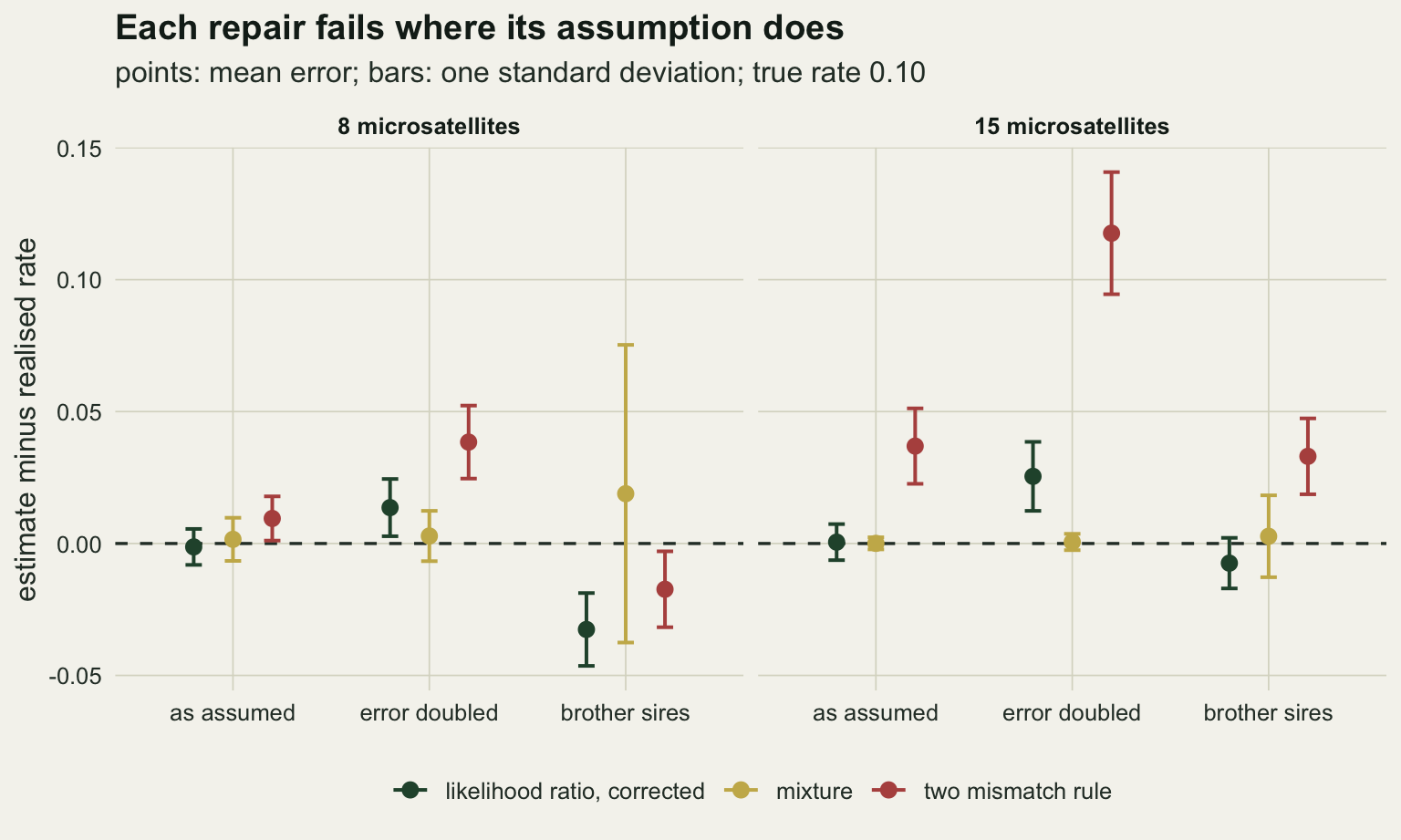
What to report
An extra-pair rate from mismatch counts is only interpretable with the panel attached. The minimum is the number of loci, their expected heterozygosity or effective number of alleles, the exclusion rule, and an error rate measured by regenotyping a sample rather than assumed. The closed form above needs more than a heterozygosity summary: it needs the allele frequencies at every locus, so publish those too (a table in the supplement is enough). With the frequencies, the rule and the error rate, a reader can compute the false exclusion rate of a fixed rule in a few lines, and decide how much of a reported rate describes the birds and how much describes the panel.
Show the histogram of mismatch counts. It costs one figure, it shows whether the two humps separate, and it is the piece of the analysis most likely to reveal related sires, because related extra-pair sires pull the second hump towards the first (a weak marker panel does the same, so read the histogram together with the exclusion probability). If the humps separate, a mixture weight is a threshold-free estimate that does not depend on the error rate. If they do not, no rule and no single estimate should be reported without a statement that related extra-pair sires would be missed.
If a likelihood ratio is used, report the simulated false exclusion and miss rates next to the threshold, and the error rate the simulation assumed. The correction is only as good as that assumption, and a calibration run once for a panel should be rerun when the error rate is remeasured.
Honest limits
The error model replaces allele calls at random. The commonest real error in microsatellites is allelic dropout, where one allele of a heterozygote fails to amplify and the individual is scored as a homozygote. Dropout is one-directional: it can turn a heterozygous chick into an apparent homozygote for an allele the social male does not carry, or hide the allele in the father that would have matched, so it produces mismatches of a specific kind (apparent opposite homozygotes) and its rate differs between loci. Hoffman and Amos 2005 measured genotyping error in a real microsatellite data set, from Antarctic fur seals, and traced its consequences for paternal exclusion. None of the closed forms here apply to dropout without rewriting the transition matrix per genotype, and the mixture would see a within-pair hump with a heavier tail at the worst loci.
Chicks were simulated one per brood. Real broods share a father, so extra-pair chicks cluster by nest and females differ in their propensity; Griffith et al. 2002 summarise how much the rate varies within and between species. Clustering would change the variance of any estimated rate and was not simulated here, and a study that reports the proportion of broods with at least one extra-pair chick is reporting a different quantity again.
Allele frequencies were known exactly. A real study estimates them from the same adults it is testing, and with rare alleles on a small sample both the likelihood ratio and the random-male mismatch probability inherit that noise. Mothers were genotyped with the same error as everyone else, but the attending female was always the true mother; egg dumping by other females is ignored.
The brother case is the extreme one: every extra-pair sire is a full brother. A real population mixes strangers, neighbours and kin, and the damage lies somewhere between the two extremes simulated here. The mixture was fitted with binomial components and a single start; on small panels with related sires, several starts and a check for a degenerate split, as in checking a mixture model, would catch some of the unstable fits, but not the overlap that causes them. Jones and Ardren 2003 review exclusion, likelihood and full-pedigree reconstruction methods, and the last of these, which uses siblings as well as the parent trio, is not tested here.
References
Jones AG, Ardren WR 2003 Molecular Ecology 12(10):2511-2523 (10.1046/j.1365-294X.2003.01928.x)
Marshall TC, Slate J, Kruuk LEB, Pemberton JM 1998 Molecular Ecology 7(5):639-655 (10.1046/j.1365-294x.1998.00374.x)
Kalinowski ST, Taper ML, Marshall TC 2007 Molecular Ecology 16(5):1099-1106 (10.1111/j.1365-294X.2007.03089.x)
Hoffman JI, Amos W 2005 Molecular Ecology 14(2):599-612 (10.1111/j.1365-294X.2004.02419.x)
Griffith SC, Owens IPF, Thuman KA 2002 Molecular Ecology 11(11):2195-2212 (10.1046/j.1365-294X.2002.01613.x)