library(ggplot2)
library(patchwork)

te_paper  <- "#f5f4ee"
te_ink    <- "#16241d"
te_body   <- "#2c3a31"
te_forest <- "#275139"
te_rust   <- "#b5534e"
te_gold   <- "#c9b458"
te_line   <- "#dad9ca"

theme_datasheet <- function() {
  theme_minimal(base_size = 12) +
    theme(plot.background  = element_rect(fill = te_paper, colour = NA),
          panel.background = element_rect(fill = te_paper, colour = NA),
          panel.grid.major = element_line(colour = te_line, linewidth = 0.3),
          panel.grid.minor = element_blank(),
          text             = element_text(colour = te_body),
          plot.title       = element_text(colour = te_ink, face = "bold"),
          plot.subtitle    = element_text(colour = te_body),
          axis.text        = element_text(colour = te_body),
          strip.text       = element_text(colour = te_ink))
}Infection rates from pooled vector samples
R
disease ecology
group testing
simulation
ecology tutorial
Pooled PCR of mosquitoes within trap-nights biases the pool MLE low and its interval undercovers. Simulating in R what randomising the pools can and cannot fix.
A West Nile virus programme runs gravid traps for Culex mosquitoes through the summer. Twenty trap-nights in a fortnight bring in a thousand females, and nobody runs a thousand PCR reactions. The mosquitoes are sorted into pools, each pool is ground up and tested once, and the report gives an infection rate per thousand mosquitoes. Two numbers are in common use. The minimum infection rate (MIR) divides the number of positive pools by the number of mosquitoes, on the assumption that a positive pool holds exactly one infected insect. The pool maximum likelihood estimate inverts the probability that a pool of m insects contains at least one infected one, 1 - (1 - p)^m, and solves for p.
Both formulas treat the insects as if each had the same chance of infection, independently of the others. In the lab they are usually sorted by species, site and night, so the insects in one pool share a trap-night. Virus activity is patchy: a trap next to a roost of infected birds on a warm night catches far more infected females than a trap on a cool night across town. The pool model sees none of that.
The known results come first, as demonstrations rather than findings. That the MIR runs low once pools are large or infection is common is textbook (Thompson 1962 derived the pool estimator for insect vectors; Gu and colleagues 2003 set out the MIR problem for mosquito programmes). The group testing literature has studied departures from independence: Hung and Swallow (1999) examined serial correlation between individuals and a dilution effect, and found that group testing coped well with the serial correlation they modelled. The correlation here is a shared infection probability for every insect caught on one trap-night, with pools nested inside nights, and at the values used below the result is not the same. What this post measures is the size of that distortion under a trap-night design, the coverage of the intervals people report, and how much of the damage goes away if the insects are mixed across the whole catch before pooling.
This site has corrected prevalence for an imperfect test, one animal at a time, in Prevalence from an imperfect test; there the correction is linear in the apparent prevalence. Estimating plant cover with point intercepts prices clustering as a design effect on a proportion, which inflates the variance and leaves the estimate unbiased. Three-level occupancy models for eDNA has several chances to miss a species, but each PCR replicate is a test of one sample, not of a mixture. Here the assay unit is a pool, and the transform from pool positivity to insect infection is not linear, so the same clustering that only widened the interval for plant cover now moves the estimate as well.
One thousand mosquitoes, twenty trap-nights
Each simulated fortnight has 20 trap-nights with 50 females each. The infection probability on trap-night j is drawn from a Beta distribution with mean p and intraclass correlation rho, so that rho is the correlation in infection status between two insects from the same trap-night; rho = 0 is the homogeneous case the pool model assumes. Pool sizes are 5, 10, 25 and 50, each dividing a trap-night’s catch, so a pool of 50 is a whole night. The design constants, including the replicate counts, were fixed before any run.
n_trap   <- 20                  # trap-nights in the fortnight
per_trap <- 50                  # females tested per trap-night
n_ins    <- n_trap * per_trap
m_set    <- c(5, 10, 25, 50)    # pool sizes, all divide per_trap
p_set    <- c(0.005, 0.01, 0.03)
rho_set  <- c(0, 0.01, 0.02, 0.05, 0.1)
n_rep    <- 2000                # datasets per cell
z_crit   <- qnorm(0.975)

draw_night_prev <- function(n_rep, p, rho) {
  if (rho == 0) return(matrix(p, n_trap, n_rep))
  s <- 1 / rho - 1
  matrix(rbeta(n_trap * n_rep, p * s, (1 - p) * s), n_trap, n_rep)
}

# pool MLE with a Wald (delta method) and a Wilson score interval, equal pools
pool_fit <- function(x, n_pool, m) {
  th <- x / n_pool
  p_hat <- 1 - (1 - th)^(1 / m)
  inner <- x > 0 & x < n_pool
  se <- ifelse(inner, sqrt(th * (1 - th) / n_pool) / m * (1 - th)^(1 / m - 1), 0)
  half <- z_crit * sqrt(th * (1 - th) / n_pool + z_crit^2 / (4 * n_pool^2))
  centre <- th + z_crit^2 / (2 * n_pool)
  w_lo <- (centre - half) / (1 + z_crit^2 / n_pool)
  w_hi <- (centre + half) / (1 + z_crit^2 / n_pool)
  list(p_hat = p_hat, wald_lo = p_hat - z_crit * se, wald_hi = p_hat + z_crit * se,
       score_lo = 1 - (1 - w_lo)^(1 / m), score_hi = 1 - (1 - w_hi)^(1 / m),
       all_pos = x == n_pool, all_neg = x == 0)
}
The Wald interval is the delta method interval on the p scale. The score interval is the Wilson interval for the pool positivity, pushed through the same monotone transform; for equal pool sizes that is the usual alternative to Wald, and the exact version is built the same way from the Clopper-Pearson interval (Hepworth 2005 extends exact intervals to pools of unequal size). When every pool is negative or every pool is positive the Wald interval collapses to a point, which is counted as a miss.
Two ways of making the pools are simulated from the same trap-night prevalences. Within-night pooling splits each night’s 50 insects into pools of m, so a pool’s positivity probability is 1 - (1 - p_j)^m for its own night. Randomised pooling first draws each insect’s infection status on its night, then deals the whole catch of a thousand into pools at random.
sim_cell <- function(p, rho, m, n_rep) {
  pj <- draw_night_prev(n_rep, p, rho)
  k <- per_trap / m; n_pool <- n_trap * k
  x_night <- matrix(rbinom(n_trap * n_rep, k, 1 - (1 - pj)^m), n_trap)
  x_within <- colSums(x_night)
  y_total <- colSums(matrix(rbinom(n_trap * n_rep, per_trap, pj), n_trap))
  x_random <- vapply(y_total, function(yy) {
    if (yy == 0) return(0L)
    length(unique((sample.int(n_ins, yy) - 1) %/% m))
  }, 1L)
  list(pj = pj, x_night = x_night, n_pool = n_pool, k = k, y_total = y_total,
       within = pool_fit(x_within, n_pool, m), random = pool_fit(x_random, n_pool, m),
       mir = x_within / n_ins)
}

summarise_cell <- function(s, p) {
  covers <- function(lo, hi, target) mean(lo <= target & hi >= target)
  w <- s$within; r <- s$random; nights <- colMeans(s$pj)
  c(bias_mle = mean(w$p_hat) / p - 1,
    bias_mle_def = mean(w$p_hat[!w$all_pos]) / p - 1,
    bias_mir = mean(s$mir) / p - 1,
    bias_rand = mean(r$p_hat[!r$all_pos]) / p - 1,
    wald_w = covers(w$wald_lo, w$wald_hi, p), score_w = covers(w$score_lo, w$score_hi, p),
    wald_r = covers(r$wald_lo, r$wald_hi, p), score_r = covers(r$score_lo, r$score_hi, p),
    wald_r_nights = covers(r$wald_lo, r$wald_hi, nights),
    wald_r_catch = covers(r$wald_lo, r$wald_hi, s$y_total / n_ins),
    all_pos = mean(w$all_pos), all_neg = mean(w$all_neg))
}

grid_cells <- expand.grid(p = p_set, rho = rho_set, m = m_set)
set.seed(1962)
grid_res <- do.call(rbind, lapply(seq_len(nrow(grid_cells)), function(i) {
  g <- grid_cells[i, ]
  summarise_cell(sim_cell(g$p, g$rho, g$m, n_rep), g$p)
}))
grid_tab <- cbind(grid_cells, grid_res)
cell <- function(p, rho, m, col) grid_tab[grid_tab$p == p & grid_tab$rho == rho & grid_tab$m == m, col]
mcse_95 <- sqrt(0.95 * 0.05 / n_rep)
The minimum infection rate is a closed form
Start where both estimators’ assumption holds, rho = 0. A pool is positive with probability 1 - (1 - p)^m, so the expected MIR is that probability divided by m, and its relative bias needs no simulation.
mir_closed <- function(p, m) (1 - (1 - p)^m) / m / p - 1
mir_gap <- max(abs(vapply(seq_len(nrow(grid_tab)), function(i)
  if (grid_tab$rho[i] == 0) grid_tab$bias_mir[i] - mir_closed(grid_tab$p[i], grid_tab$m[i]) else 0, 0)))
homog <- grid_tab[grid_tab$rho == 0, ]
mle_homog_max <- max(abs(homog$bias_mle_def))
The simulated MIR bias matches the closed form to 0.004 over the homogeneous cells. At a pool size of 50 the MIR is 11 per cent low at p = 0.005, 21 per cent low at p = 0.01 and 48 per cent low at p = 0.03; at a pool size of 5 the three figures are 1.0, 2.0 and 5.8 per cent. The pool MLE, averaged over the datasets in which at least one pool was negative, is within 5.9 per cent of the truth in every homogeneous cell, running slightly high at the largest pools.
The exception needs a sentence, because it looks like a large bias. At p = 0.03 and pools of 50, 0.9 per cent of fortnights return every pool positive, the estimate is then exactly 1, and the plain average of the estimates is +0.37 in relative terms. That is the known upward small-sample bias of the pool MLE, and here it lives almost entirely in those all-positive fortnights, which a programme would report as a lower bound rather than a rate.
mir_lines <- expand.grid(m = seq(1, 50, by = 0.5), p = p_set)
mir_lines$bias <- mir_closed(mir_lines$p, mir_lines$m)
p_lab <- function(p) factor(sprintf("p = %s", p), levels = sprintf("p = %s", p_set))
mir_lines$prev <- p_lab(mir_lines$p); homog$prev <- p_lab(homog$p)
ggplot() +
  geom_hline(yintercept = 0, colour = te_body, linetype = "dashed", linewidth = 0.5) +
  geom_line(data = mir_lines, aes(m, bias, colour = prev), linewidth = 0.9) +
  geom_point(data = homog, aes(m, bias_mir, colour = prev), size = 2.6) +
  geom_point(data = homog, aes(m, bias_mle_def, colour = prev), shape = 21,
             fill = te_paper, size = 2.6, stroke = 0.9) +
  scale_colour_manual(values = c(te_gold, te_forest, te_rust), name = NULL) +
  scale_x_continuous(breaks = m_set) +
  labs(x = "insects per pool", y = "relative bias",
       title = "The MIR falls behind as pools grow",
       subtitle = "filled: MIR, open: pool MLE (all-positive datasets left out)") +
  theme_datasheet() + theme(legend.position = "bottom")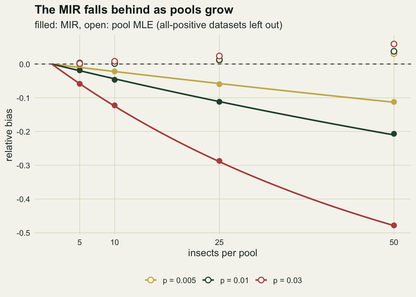
Pooling within trap-nights biases the pool estimate
Once prevalence varies between trap-nights and pools are formed within a night, the probability that a pool is positive is the average of 1 - (1 - p_j)^m over nights, and 1 - (1 - p)^m is concave in p, so that average is below the value at the mean. Under the Beta model the average has a closed form, 1 - B(a, b + m) / B(a, b), and the pool MLE converges to the p that reproduces it. That gives the bias without simulation, and the simulation is a check on it.
pool_limit_bias <- function(p, rho, m) {
  if (rho == 0) return(0)
  s <- 1 / rho - 1; a <- p * s; b <- (1 - p) * s
  theta <- 1 - exp(lbeta(a, b + m) - lbeta(a, b))
  (1 - (1 - theta)^(1 / m)) / p - 1
}
grid_tab$bias_closed <- mapply(pool_limit_bias, grid_tab$p, grid_tab$rho, grid_tab$m)
chk <- grid_tab[grid_tab$rho > 0 & grid_tab$p >= 0.01, ]
bias_gap <- max(abs(chk$bias_mle_def - chk$bias_closed))
gap_at <- chk[which.max(abs(chk$bias_mle_def - chk$bias_closed)), ]
chk5 <- grid_tab[grid_tab$rho > 0 & grid_tab$p == 0.005, ]
bias_gap5 <- max(abs(chk5$bias_mle_def - chk5$bias_closed))
rand_bias_max <- max(abs(grid_tab$bias_rand[grid_tab$p >= 0.01]))
rand_bias_max_m25 <- max(abs(grid_tab$bias_rand[grid_tab$p >= 0.01 & grid_tab$m <= 25]))
s_02 <- 1 / 0.02 - 1
share_quiet <- pbeta(0.001, 0.01 * s_02, 0.99 * s_02)
share_hot <- 1 - pbeta(0.03, 0.01 * s_02, 0.99 * s_02)
For p = 0.01 and 0.03 the simulated bias and the closed form agree to 0.052 in relative terms across all heterogeneous cells, the largest gap at p = 0.03, rho = 0.01 and pools of 50, where the small-sample upward bias of the estimator pulls the simulated value above the limit (simulated -0.135, limit -0.187), and to 0.027 at p = 0.005, where fortnights with no positive pool at all are common and the small-sample behaviour of the estimator adds to the limit. The limit hardly depends on p: at rho = 0.02 it is -0.081, -0.185 and -0.306 at pools of 10, 25 and 50 for p = 0.01, and -0.081, -0.185 and -0.305 for p = 0.03. At rho = 0.1 the pool of 50 reports 0.35 of the true rate. The MIR carries this bias on top of its own: at rho = 0.02 and pools of 50 it is -0.41 in relative terms at p = 0.01.
Randomising the pools removes it. With the catch dealt into pools at random, the largest relative bias of the pool MLE over the cells with p of 0.01 or 0.03 is 0.028 for pools of up to 25, and 0.068 once pools of 50 are included, where the small-sample upward bias of the previous section appears whatever the value of rho. The pool then mixes nights, and the pool positivity depends on the realised proportion of infected insects in the catch, not on how they were grouped.
het <- grid_tab[grid_tab$rho > 0 & grid_tab$p >= 0.01, ]
het$prev <- p_lab(het$p)
het$rho_lab <- factor(sprintf("rho = %s", het$rho), levels = sprintf("rho = %s", rho_set[-1]))
bias_lines <- expand.grid(m = 1:50, p = c(0.01, 0.03), rho = rho_set[-1])
bias_lines$bias <- mapply(pool_limit_bias, bias_lines$p, bias_lines$rho, bias_lines$m)
bias_lines$prev <- p_lab(bias_lines$p)
bias_lines$rho_lab <- factor(sprintf("rho = %s", bias_lines$rho), levels = levels(het$rho_lab))
ggplot() +
  geom_hline(yintercept = 0, colour = te_body, linetype = "dashed", linewidth = 0.5) +
  geom_line(data = bias_lines, aes(m, bias, colour = rho_lab), linewidth = 0.8) +
  geom_point(data = het, aes(m, bias_mle_def, colour = rho_lab), size = 2.4) +
  facet_wrap(~ prev) +
  scale_colour_manual(values = c(te_gold, te_forest, te_rust, te_ink), name = NULL) +
  scale_x_continuous(breaks = m_set) +
  labs(x = "insects per pool", y = "relative bias of the pool MLE",
       title = "Within-night pools pull the estimate down",
       subtitle = "lines: 1 - B(a, b + m) / B(a, b) limit, points: 2000 fortnights") +
  theme_datasheet() + theme(legend.position = "bottom")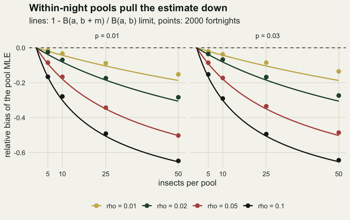
The reported interval does not see it
The bias would matter less if the interval widened to cover it. It does not, because the binomial pool model thinks each pool is an independent trial with a common probability, and it has no term for the between-night variation, so the interval neither re-centres nor widens for it.
cov_w <- grid_tab[grid_tab$p >= 0.01, ]
wald_homog <- range(cov_w$wald_w[cov_w$rho == 0])
score_homog <- range(cov_w$score_w[cov_w$rho == 0])
neg_max <- max(grid_tab$all_neg[grid_tab$p == 0.005 & grid_tab$rho == 0.1])
neg_homog <- max(grid_tab$all_neg[grid_tab$p == 0.005 & grid_tab$rho == 0])
In the homogeneous cells with p of 0.01 or 0.03 the Wald interval covers in 0.910 to 0.956 of fortnights and the score interval in 0.941 to 0.970, with a Monte Carlo standard error of 0.005 near 0.95. The Wald shortfall at p = 0.01 is the usual behaviour of a Wald interval built on a few positive pools.
With within-night pools and rho = 0.02, the Wald interval at p = 0.03 covers in 0.816, 0.857, 0.800 and 0.606 of fortnights at pools of 5, 10, 25 and 50, and the score interval in 0.856, 0.864, 0.797 and 0.606. The decline with pool size is not smooth at this rho: the small pools lose some coverage too, and the large step comes at pools of 50, where each night is a single pool. At p = 0.01 the Wald figures are 0.827, 0.800, 0.724 and 0.757, but the score interval holds up better, at 0.882, 0.906, 0.931 and 0.890. That is not a repair: with few positive pools the score interval is long on the upper side, and the extra length happens to reach a truth that sits above the biased centre. At p = 0.03 there are enough positive pools for the score and Wald intervals to be nearly the same, and the rescue is gone.
At rho = 0.1 and pools of 50 the Wald interval covers in 0.195 of fortnights at p = 0.01 and 0.027 at p = 0.03. At p = 0.005 and rho = 0.1 up to 18.7 per cent of fortnights have no positive pool at all (against at most 0.7 per cent with rho = 0), because the virus is confined to a few nights and the others contribute nothing.
cov_long <- rbind(
  data.frame(cov_w[, c("p", "rho", "m")], interval = "Wald", coverage = cov_w$wald_w),
  data.frame(cov_w[, c("p", "rho", "m")], interval = "score", coverage = cov_w$score_w))
cov_long$prev <- p_lab(cov_long$p)
cov_long$interval <- factor(cov_long$interval, levels = c("Wald", "score"))
cov_long$rho_lab <- factor(sprintf("rho = %s", cov_long$rho), levels = sprintf("rho = %s", rho_set))
ggplot(cov_long, aes(m, coverage, colour = rho_lab, linetype = rho_lab)) +
  annotate("rect", xmin = -Inf, xmax = Inf, ymin = 0.95 - 2 * mcse_95,
           ymax = 0.95 + 2 * mcse_95, fill = te_line, alpha = 0.8) +
  geom_line(linewidth = 0.8) + geom_point(size = 2) +
  facet_grid(interval ~ prev) +
  scale_colour_manual(values = c(te_body, te_gold, te_forest, te_rust, te_ink), name = NULL) +
  scale_linetype_manual(values = c("dashed", "solid", "solid", "solid", "solid"), name = NULL) +
  scale_x_continuous(breaks = m_set) +
  scale_y_continuous(limits = c(0, 1)) +
  guides(colour = guide_legend(nrow = 1), linetype = guide_legend(nrow = 1)) +
  labs(x = "insects per pool", y = "coverage of the true rate",
       title = "Coverage falls as nights differ and pools grow",
       subtitle = "within-night pools; rho = 0 dashed") +
  theme_datasheet() + theme(legend.position = "bottom")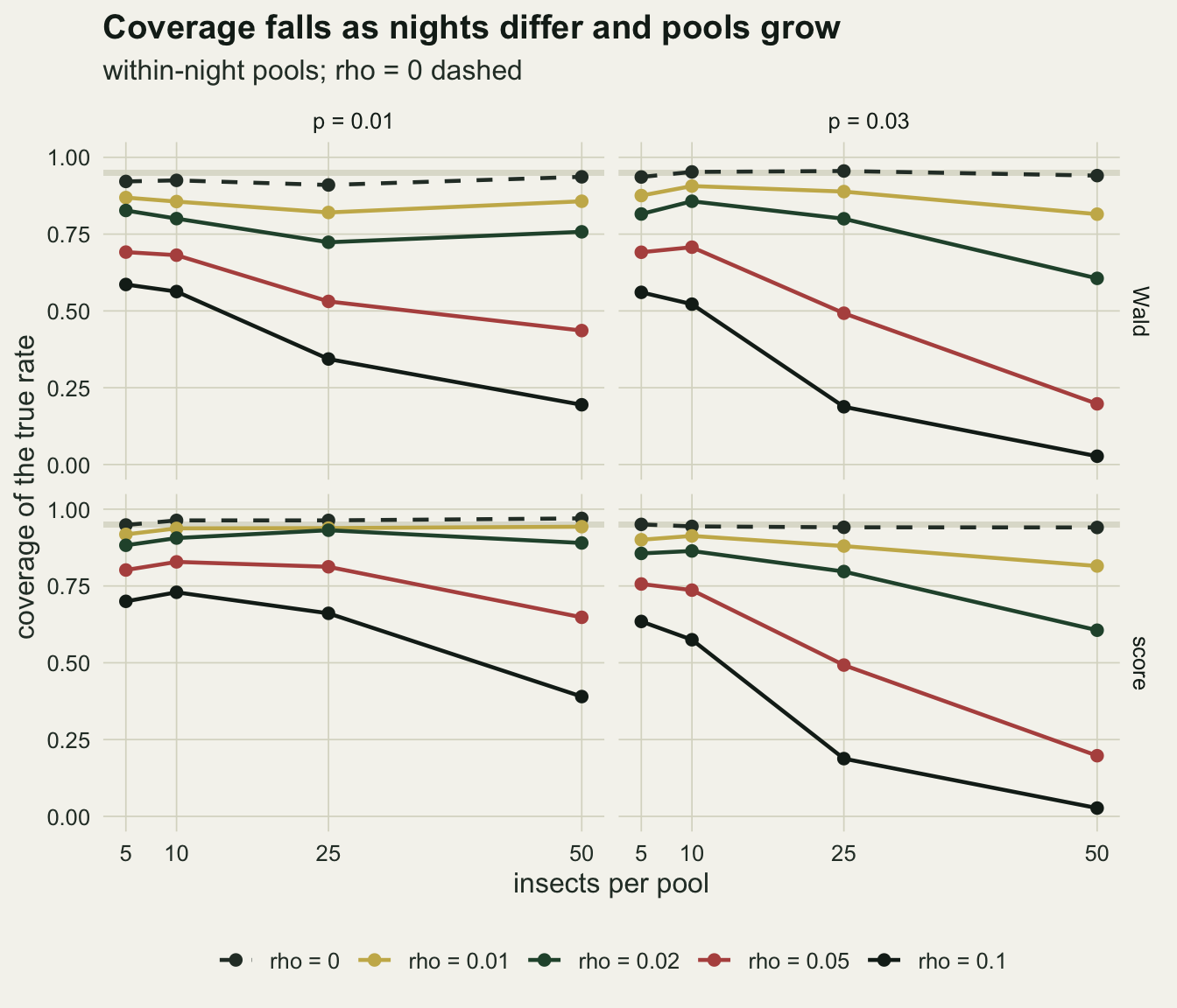
Randomising fixes the estimate, not the population interval
Randomised pooling removed the bias. Whether it restores coverage depends on what the interval is for, and there are three candidates. The narrowest is the realised proportion of infected insects in the thousand that were caught. The next is the infection probability averaged over the 20 nights that were sampled, what an unlimited catch on exactly those nights would show; it differs from the realised proportion by the binomial sampling of insects within nights. The widest is the mean infection rate p across all the nights the fortnight could have been trapped, which also carries the between-night variation of which nights happened to be sampled; an individual PCR on every insect would carry that too. The pool model’s variance is binomial, which matches the middle target. With the Beta model the extra variance for the population rate is p(1 - p) rho / 20, so the expected Wald coverage for the population rate is a one-line calculation to set beside the simulation.
wald_predicted <- function(p, rho, m) {
  k <- per_trap / m; n_pool <- n_trap * k
  theta <- 1 - (1 - p)^m
  v_pool <- theta * (1 - theta) / n_pool / m^2 * (1 - theta)^(2 / m - 2)
  v_night <- p * (1 - p) * rho / n_trap
  2 * pnorm(z_crit * sqrt(v_pool / (v_pool + v_night))) - 1
}
grid_tab$wald_pred <- mapply(wald_predicted, grid_tab$p, grid_tab$rho, grid_tab$m)
rnd <- grid_tab[grid_tab$p >= 0.01 & grid_tab$all_pos < 0.001, ]
nights_range <- range(rnd$wald_r_nights[rnd$p == 0.03])
nights_range01 <- range(rnd$wald_r_nights[rnd$p == 0.01])
pred_gap <- max(abs(rnd$wald_r - rnd$wald_pred)[rnd$p == 0.03])
catch_range <- range(rnd$wald_r_catch)
wr01 <- sapply(m_set, function(mm) cell(0.01, 0.02, mm, "wald_r"))
wr03 <- sapply(m_set, function(mm) cell(0.03, 0.02, mm, "wald_r"))
wp03 <- sapply(m_set, function(mm) cell(0.03, 0.02, mm, "wald_pred"))
For the mean infection probability on the sampled nights the randomised Wald interval covers in 0.922 to 0.955 of fortnights across all rho and pool sizes at p = 0.03, and 0.904 to 0.944 at p = 0.01, where the Wald interval’s own small-count shortfall remains. For the realised proportion in the catch it runs at or above the nominal level, covering in 0.951 to 1.000 of fortnights over the same cells, because once the catch is fixed only the random dealing into pools is left to vary. For the population rate p it is a different story. At rho = 0.02 and p = 0.03 the randomised Wald interval covers in 0.814, 0.854 and 0.893 of fortnights at pools of 5, 10 and 25, against predicted values of 0.841, 0.848 and 0.870; at rho = 0.1 the same three figures are 0.554, 0.605 and 0.659. Across the p = 0.03 cells the prediction and the simulation differ by at most 0.048; the prediction is a normal approximation and ignores the Wald interval’s own shortfall with few positive pools, which is larger at p = 0.01.
The prediction also explains a detail that looks backwards: at p = 0.03 and rho = 0.02 the population coverage under randomised pooling rises with pool size, 0.814, 0.854, 0.893 and 0.888 at pools of 5 to 50 (predicted 0.841, 0.848, 0.870 and 0.899), levelling off after 25, because the between-night variance is fixed while larger pools lose information and widen the interval. At p = 0.01 the simulated figures, 0.802, 0.818, 0.782 and 0.862, do not rise steadily: the Wald interval’s own small-count behaviour is added on top of the pattern. Mixing the insects cannot tell the analysis how variable the nights were. Once the pools are mixed, nothing in the data measures it.
A trap-night bootstrap sees the nights and keeps the bias
The other repair keeps the within-night pools and resamples trap-nights: draw 20 nights with replacement, carry each night’s positive-pool count with it, recompute the pool MLE, and take the percentile interval over 500 resamples. It measures the between-night variation directly. With 20 nights the question is also whether it holds its level when there is no variation at all. The bootstrap is slower, so it runs on 1000 fortnights per cell, for two prevalences and three values of rho.
n_rep_boot <- 1000
n_boot <- 500
boot_cell <- function(p, rho, m) {
  s <- sim_cell(p, rho, m, n_rep_boot)
  hits <- vapply(seq_len(n_rep_boot), function(r) {
    idx <- matrix(sample.int(n_trap, n_trap * n_boot, replace = TRUE), n_trap)
    x_b <- colSums(matrix(s$x_night[idx, r], n_trap))
    q <- quantile(1 - (1 - x_b / s$n_pool)^(1 / m), c(0.025, 0.975), names = FALSE)
    q[1] <= p && q[2] >= p
  }, TRUE)
  c(boot = mean(hits), wald = mean(s$within$wald_lo <= p & s$within$wald_hi >= p))
}
boot_cells <- expand.grid(p = c(0.01, 0.03), rho = c(0, 0.02, 0.05), m = m_set)
set.seed(2003)
boot_tab <- cbind(boot_cells, t(mapply(boot_cell, boot_cells$p, boot_cells$rho, boot_cells$m)))
bcell <- function(p, rho, m, col = "boot") boot_tab[boot_tab$p == p & boot_tab$rho == rho & boot_tab$m == m, col]
boot_homog <- range(boot_tab$boot[boot_tab$rho == 0])
mcse_boot <- sqrt(0.95 * 0.05 / n_rep_boot)
pop_cov <- grid_tab[grid_tab$rho > 0 & grid_tab$p >= 0.01, ]
pop_best <- max(unlist(pop_cov[, c("wald_w", "score_w", "wald_r", "score_r")]), boot_tab$boot[boot_tab$rho > 0])
boot_vs_rand_se <- sqrt(bcell(0.03, 0.02, 5) * (1 - bcell(0.03, 0.02, 5)) / n_rep_boot +
  cell(0.03, 0.02, 25, "wald_r") * (1 - cell(0.03, 0.02, 25, "wald_r")) / n_rep)
With rho = 0 the bootstrap interval covers in 0.910 to 0.940 of fortnights over the eight cells, a Monte Carlo standard error of 0.007: a percentile bootstrap over 20 clusters runs a little short even when the clusters are identical. At rho = 0.02 it covers in 0.906, 0.888, 0.853 and 0.772 at p = 0.03 for pools of 5 to 50, where the Wald interval on the same fortnights covers in 0.817, 0.842, 0.819 and 0.610. At p = 0.01 and rho = 0.02 the bootstrap coverage goes from 0.875 with pools of 5 to 0.829 with pools of 50. At p = 0.03 and rho = 0.05 it reaches 0.865 with pools of 5 and 0.359 with pools of 50.
The pattern is the one the bias section predicts. The bootstrap gets the width from the nights, but it resamples an estimator whose centre has already moved, so at p = 0.03 its coverage falls with pool size as the bias grows. At p = 0.01 and rho = 0.02 it is nearly flat from pools of 5 to 25 (0.875, 0.867 and 0.868) while the bias limit moves from -0.038 to -0.185, and drops only at pools of 50.
At p = 0.03 and rho = 0.02, small pools inside nights with a bootstrap over nights are among the best of the analyses measured here: 0.906 at pools of 5, against 0.893 for randomised pools of 25, a difference of 0.013 with a Monte Carlo standard error of 0.012, so the two are not clearly ranked. At p = 0.01 and rho = 0.02 the within-night score interval does as well as the bootstrap at pools of 5 (0.882 against 0.875) and better at pools of 10 to 50 (0.906, 0.931 and 0.890 against 0.867, 0.868 and 0.829), for the accidental reason given earlier. No analysis at p of 0.01 or 0.03 reaches 0.95 at a nonzero rho; the highest coverage of the population rate is 0.943, from the within-night score interval at p = 0.01, rho = 0.01 and pools of 50. The lowest prevalence is left out of that statement on purpose, so here it is: at p = 0.005 the within-night score interval covers in 0.982 at rho = 0.01 and 0.964 at rho = 0.02 with pools of 50, but it already covers in 0.956 to 0.972 with rho = 0 there, and its centre carries the same within-night bias; it is the long upper side at a handful of positive pools, not a repair.
rep_rows <- lapply(c(0, 0.02, 0.05), function(rr) {
  g <- grid_tab[grid_tab$p == 0.03 & grid_tab$rho == rr, ]
  b <- boot_tab[boot_tab$p == 0.03 & boot_tab$rho == rr, ]
  rbind(data.frame(rho = rr, m = g$m, analysis = "within-night Wald", coverage = g$wald_w),
        data.frame(rho = rr, m = b$m, analysis = "trap-night bootstrap", coverage = b$boot),
        data.frame(rho = rr, m = g$m, analysis = "randomised Wald", coverage = g$wald_r),
        data.frame(rho = rr, m = g$m, analysis = "randomised, predicted", coverage = g$wald_pred))
})
rep_df <- do.call(rbind, rep_rows)
rep_df$analysis <- factor(rep_df$analysis, levels = c("within-night Wald", "trap-night bootstrap",
                                                      "randomised Wald", "randomised, predicted"))
rep_df$rho_lab <- factor(sprintf("rho = %s", rep_df$rho), levels = sprintf("rho = %s", c(0, 0.02, 0.05)))
ggplot(rep_df, aes(m, coverage, colour = analysis, linetype = analysis)) +
  annotate("rect", xmin = -Inf, xmax = Inf, ymin = 0.95 - 2 * mcse_95,
           ymax = 0.95 + 2 * mcse_95, fill = te_line, alpha = 0.8) +
  geom_line(linewidth = 0.8) + geom_point(size = 2) +
  facet_wrap(~ rho_lab) +
  scale_colour_manual(values = c(te_rust, te_forest, te_gold, te_ink), name = NULL) +
  scale_linetype_manual(values = c("solid", "solid", "solid", "dashed"), name = NULL) +
  scale_x_continuous(breaks = m_set) +
  scale_y_continuous(limits = c(0, 1)) +
  guides(colour = guide_legend(nrow = 2)) +
  labs(x = "insects per pool", y = "coverage of the population rate",
       title = "No analysis of pooled data restores 0.95 once nights differ",
       subtitle = "p = 0.03; grey band: 0.95 plus or minus two Monte Carlo standard errors") +
  theme_datasheet() + theme(legend.position = "bottom")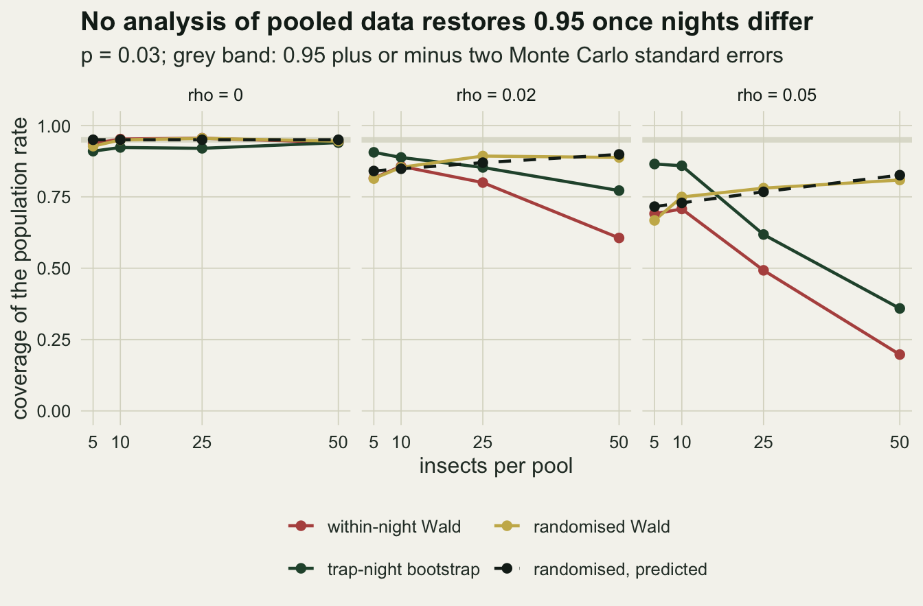
Does the Beta shape drive the bias?
The closed form depends on the whole distribution of p_j through E[(1 - p_j)^m], so a different distribution with the same mean and the same rho need not give the same bias. A logit-normal night effect is the other common choice. Matching its mean and variance to the Beta at p = 0.01 and rho = 0.02 and rerunning the within-night pools is a check on how much of the result belongs to the Beta.
z_nodes <- qnorm(ppoints(4000))
ln_moments <- function(par) {
  v <- plogis(par[1] + exp(par[2]) * z_nodes)
  c(mean(v), var(v))
}
p_ln <- 0.01; rho_ln <- 0.02
target <- c(p_ln, p_ln * (1 - p_ln) * rho_ln)
ln_fit <- optim(c(qlogis(p_ln), 0), function(par) sum(((ln_moments(par) - target) / target)^2),
                control = list(reltol = 1e-12, maxit = 5000))
ln_mu <- ln_fit$par[1]; ln_sd <- exp(ln_fit$par[2])
ln_match <- max(abs(ln_moments(ln_fit$par) / target - 1))
ln_limit <- function(m) {
  theta <- 1 - mean((1 - plogis(ln_mu + ln_sd * z_nodes))^m)
  (1 - (1 - theta)^(1 / m)) / p_ln - 1
}
set.seed(1996)
ln_res <- t(vapply(c(10, 25, 50), function(m) {
  pj <- matrix(plogis(ln_mu + ln_sd * rnorm(n_trap * n_rep)), n_trap)
  k <- per_trap / m; n_pool <- n_trap * k
  fit <- pool_fit(colSums(matrix(rbinom(n_trap * n_rep, k, 1 - (1 - pj)^m), n_trap)), n_pool, m)
  c(m = m, limit = ln_limit(m), bias = mean(fit$p_hat[!fit$all_pos]) / p_ln - 1,
    wald = mean(fit$wald_lo <= p_ln & fit$wald_hi >= p_ln))
}, numeric(4)))
The logit-normal with mean 0.010 and the same variance as the Beta has a logit-scale standard deviation of 1.10 (moments matched to a relative error of 8.2e-07). Its limiting relative bias is -0.076, -0.161 and -0.254 at pools of 10, 25 and 50, against -0.081, -0.185 and -0.306 under the Beta; simulated, it is -0.061, -0.144 and -0.226, with Wald coverage 0.836, 0.774 and 0.817. The Beta limit is 1.20 times the logit-normal one at pools of 50, so the shape of the night distribution moves the size of the bias by a noticeable margin; the direction of the bias, its growth with pool size and a loss of coverage are the same under both, at this one setting.
What to report
Report the pool MLE, not the MIR, and give the pool sizes and the number of pools alongside it. The MIR bias is arithmetic and grows with pool size and prevalence; at pools of 50 and p = 0.03 it is 48 per cent even with no heterogeneity at all.
Say how pools were formed. “Pools of up to 50 by species, site and night” and “pools formed at random from the fortnight’s catch” are different designs, and the first one’s estimate is low by an amount set by the between-night correlation and the pool size, 31 per cent at rho = 0.02 and pools of 50 under the model here. If pools must follow nights for logistic reasons, keep them small.
Say which rate the interval is for. An interval from randomised pools is an interval for the infection rate on the nights that were trapped, not for the vector population across the fortnight’s possible nights. A statement about the population needs trap-nights as the replicates, and with within-night pools the trap-night bootstrap is the analysis that looks at them; the bootstrap inherits the within-night bias, so it comes nearest with small pools and still falls short (0.906 at pools of 5, rho = 0.02 and p = 0.03), and with pools of 50 no analysis at p of 0.01 or 0.03 reaches 0.95 for the population rate (at p = 0.005 the over-long score interval does, at rho of 0.01 and 0.02).
Report the number of trap-nights and the number of nights with at least one positive pool. Together they tell a reader whether the virus signal came from a few hot nights, which is exactly the situation in which every interval above is too narrow.
Honest limits
Everything here has equal pool sizes, a perfect assay and a fixed catch of 50 per night. Real catches vary, so pools of unequal size are common, the pool MLE then has no closed form and needs a numerical fit (Hepworth 2005 treats the intervals), and nights with large catches contribute more pools and more weight. The direction of the within-night bias does not depend on equal sizes, because it comes from the concavity of the pool transform, but its size will differ. A PCR with imperfect sensitivity on a pool of 50 is a separate problem with a dilution effect that grows with pool size; it would add a second downward pull, not simulated here.
The between-night variation is a single Beta or logit-normal draw per night, independent across nights. Real arbovirus activity clusters in space and builds through a season, so neighbouring nights and neighbouring traps are correlated, and twenty nights are then worth fewer than twenty independent ones. The bootstrap here resamples nights as if they were independent, which is the favourable case for it.
The rho values used are assumptions, not estimates from surveillance data. A trap-night correlation of 0.02 with a mean infection rate of 0.01 already puts 25 per cent of nights below one infected insect per thousand and 8.4 per cent above three per cent; whether real programmes sit nearer 0.01 or 0.1 has to come from their own trap-level data, which pooled testing within nights at pools of 50 cannot supply.
The randomised design assumes the lab can mix the fortnight’s catch before testing. That discards the night and site information a programme uses to locate virus activity, which is often the point of the surveillance, and many programmes will reasonably keep night-level pools and accept the bias. The post measures that trade rather than resolving it.
Only the percentile bootstrap was run. Bias-corrected or studentised versions could do better at 20 clusters, and a beta-binomial model of pool counts per night (possible only with several pools per night) would estimate the between-night variation directly. Neither was measured.
References
Thompson KH 1962 Biometrics 18(4):568 (10.2307/2527902)
Gu W, Lampman R, Novak RJ 2003 Journal of Medical Entomology 40(5):595-596 (10.1603/0022-2585-40.5.595)
Hung M, Swallow WH 1999 Biometrics 55(1):231-237 (10.1111/j.0006-341X.1999.00231.x)
Hepworth G 2005 Journal of Agricultural, Biological, and Environmental Statistics 10(4):478-497 (10.1198/108571105X81698)