library(ggplot2)

te_paper  <- "#f5f4ee"
te_ink    <- "#16241d"
te_body   <- "#2c3a31"
te_forest <- "#275139"
te_rust   <- "#b5534e"
te_gold   <- "#c9b458"
te_line   <- "#dad9ca"

theme_datasheet <- function() {
  theme_minimal(base_size = 12) +
    theme(plot.background  = element_rect(fill = te_paper, colour = NA),
          panel.background = element_rect(fill = te_paper, colour = NA),
          panel.grid.major = element_line(colour = te_line, linewidth = 0.3),
          panel.grid.minor = element_blank(),
          text             = element_text(colour = te_body),
          plot.title       = element_text(colour = te_ink, face = "bold"),
          plot.subtitle    = element_text(colour = te_body),
          axis.text        = element_text(colour = te_body),
          strip.text       = element_text(colour = te_ink))
}Two imperfect tests and no gold standard
R
disease ecology
diagnostic tests
latent class models
simulation
ecology tutorial
Fitting the Hui-Walter latent class model in R: why Wald intervals undercover, when profile intervals keep coverage, and why test dependence cannot be seen.
A wildlife health team has blood from wild boar shot in two hunting districts, 800 animals from each. Every serum goes through two assays for the same virus: a laboratory ELISA and a cheaper rapid test that a hunter could run in the field. Neither is a gold standard. No panel of animals of known status exists for boar, the validation figures that came with the kits were produced in domestic pigs, and the district where the virus has been circulating for years is plainly not the same population as the one where it arrived last winter. The team wants prevalence in both districts and the sensitivity and specificity of both tests, and it has nothing to anchor them to except the two tests themselves.
Prevalence from an imperfect test corrects apparent prevalence with sensitivity and specificity taken from a validation study, and it closes by pointing in this direction: two imperfect tests applied to the same animals in two populations with different prevalences identify all the parameters without any validation panel. That is the Hui and Walter (1980) model, and this post fits it from scratch. The model is a latent class model with two classes, infected and not, and the problems it runs into are the ones this site has met in other latent class settings. Checking a mixture model opens with the question of which optimum a run found; False positives in occupancy models has a label swap that leaves two answers fitting the data alike; Checking a distance sampling model names the direction in which unmodelled heterogeneity pulls an estimate of the hidden class, and correlated misses between two tests are the same mechanism.
Two results used here are known and are demonstrated, not discovered. Hui and Walter showed that two tests and two populations give exactly as many independent cell frequencies as there are parameters. Vacek (1985) showed that if the tests err together, which two assays aimed at the same antibody can be expected to do, the estimates are biased and the fit gives no sign of it. A third is close to arithmetic too: how often the best optimum sits on the boundary of the parameter space follows from the expected information of the model, and the post prints that prediction next to the simulated share. What this post measures, and what no formula here gives, is what happens to the intervals and to a single analysis on data of realistic size: whether Wald and profile likelihood intervals keep their coverage, why the Wald interval loses it, what dependence does to the coverage of an interval that looks well determined, and how often a plain optim run stops at a false optimum.
Four cells, two populations, six parameters
Each animal gives one of four results: positive on both tests, positive on the ELISA only, positive on the rapid test only, negative on both. Among infected animals the chance of each pattern is a product of sensitivities, among uninfected animals a product of specificities, and the population’s prevalence mixes the two. Conditional independence, the assumption that the two tests err independently given true status, is what makes the products valid. The design constants below were fixed before any simulation was run: sensitivities of 0.85 and 0.75, specificities of 0.95 and 0.98, prevalence 0.30 in the older district. They are illustrative values, not published figures for any real assay.
se_true   <- c(0.85, 0.75)       # ELISA, rapid test
sp_true   <- c(0.95, 0.98)
prev1     <- 0.30                # older district
prev2_set <- c(0.25, 0.20, 0.05) # newer district: gaps 0.05, 0.10, 0.25
n_set     <- c(200, 800)         # animals per district
n_rep     <- 300
n_rand    <- 10                  # random starts per dataset
crit      <- qchisq(0.95, 1)
miss_tol  <- 1                 # nll units that count as a missed optimum

# cell order: ++, +-, -+, --; cov_pos and cov_neg are conditional covariances
cell_prob <- function(prev, se1, se2, sp1, sp2, cov_pos = 0, cov_neg = 0) {
  inf <- c(se1 * se2 + cov_pos, se1 * (1 - se2) - cov_pos,
           (1 - se1) * se2 - cov_pos, (1 - se1) * (1 - se2) + cov_pos)
  uninf <- c((1 - sp1) * (1 - sp2) + cov_neg, (1 - sp1) * sp2 - cov_neg,
             sp1 * (1 - sp2) - cov_neg, sp1 * sp2 + cov_neg)
  prev * inf + (1 - prev) * uninf
}
Each district’s four cell probabilities sum to one, so each district contributes three free frequencies, six in total. The model has six parameters: two prevalences, two sensitivities, two specificities. The fitter works on the logit scale so that optim never proposes a probability outside zero and one, and it carries its analytic gradient, which makes each fit a few milliseconds. Fixing one parameter and maximising over the other five gives the profile likelihood used later for intervals.
# parameter order on the logit scale: prev1, prev2, se1, se2, sp1, sp2
hw_nll <- function(theta, y1, y2) {
  q <- plogis(theta)
  -sum(y1 * log(cell_prob(q[1], q[3], q[4], q[5], q[6]))) -
    sum(y2 * log(cell_prob(q[2], q[3], q[4], q[5], q[6])))
}
hw_grad <- function(theta, y1, y2) {
  q <- plogis(theta); se1 <- q[3]; se2 <- q[4]; sp1 <- q[5]; sp2 <- q[6]
  inf   <- c(se1 * se2, se1 * (1 - se2), (1 - se1) * se2, (1 - se1) * (1 - se2))
  uninf <- c((1 - sp1) * (1 - sp2), (1 - sp1) * sp2, sp1 * (1 - sp2), sp1 * sp2)
  d_se1 <- c(se2, 1 - se2, -se2, -(1 - se2)); d_se2 <- c(se1, -se1, 1 - se1, -(1 - se1))
  d_sp1 <- c(-(1 - sp2), -sp2, 1 - sp2, sp2); d_sp2 <- c(-(1 - sp1), 1 - sp1, -sp1, sp1)
  g <- numeric(6)
  for (k in 1:2) {
    pk <- q[k]; yk <- if (k == 1) y1 else y2
    w  <- -yk / (pk * inf + (1 - pk) * uninf)
    g[k]   <- sum(w * (inf - uninf))
    g[3:6] <- g[3:6] + c(sum(w * pk * d_se1), sum(w * pk * d_se2),
                         sum(w * (1 - pk) * d_sp1), sum(w * (1 - pk) * d_sp2))
  }
  g * q * (1 - q)
}
hw_fit <- function(start, y1, y2, fixed = 0, value = NA) {
  if (fixed == 0) {
    o <- optim(qlogis(start), hw_nll, hw_grad, y1 = y1, y2 = y2,
               method = "BFGS", control = list(maxit = 1000))
    return(c(plogis(o$par), nll = o$value))
  }
  full <- function(th5) append(th5, qlogis(value), after = fixed - 1)
  o <- optim(qlogis(start[-fixed]), function(th5) hw_nll(full(th5), y1, y2),
             function(th5) hw_grad(full(th5), y1, y2)[-fixed],
             method = "BFGS", control = list(maxit = 1000))
  o$value
}
start_default <- c(0.2, 0.2, 0.8, 0.8, 0.9, 0.9)
start_other   <- c(0.3, 0.6, 0.8, 0.8, 0.9, 0.9)
start_random  <- function() c(runif(2, 0.01, 0.6), runif(4, 0.5, 0.99))

# check the analytic gradient against central differences
theta_chk <- qlogis(c(0.3, 0.1, 0.8, 0.7, 0.9, 0.95))
y_chk1 <- c(120, 60, 40, 580); y_chk2 <- c(20, 30, 40, 710)
num_grad <- sapply(1:6, function(j) {
  e <- replace(numeric(6), j, 1e-6)
  (hw_nll(theta_chk + e, y_chk1, y_chk2) - hw_nll(theta_chk - e, y_chk1, y_chk2)) / 2e-6
})
grad_err <- max(abs(num_grad - hw_grad(theta_chk, y_chk1, y_chk2)))
The analytic gradient agrees with central differences to 1.51e-07, so the fits below are not steered by a coding slip.
set.seed(4102)
p_old <- cell_prob(prev1, se_true[1], se_true[2], sp_true[1], sp_true[2])
p_new <- cell_prob(0.05, se_true[1], se_true[2], sp_true[1], sp_true[2])
y_old <- rmultinom(1, 800, p_old)[, 1]
y_new <- rmultinom(1, 800, p_new)[, 1]
fit_one <- hw_fit(start_default, y_old, y_new)
fitted_gap <- max(abs(c(cell_prob(fit_one[1], fit_one[3], fit_one[4], fit_one[5], fit_one[6]) - y_old / 800,
                        cell_prob(fit_one[2], fit_one[3], fit_one[4], fit_one[5], fit_one[6]) - y_new / 800)))
rbind(old = y_old, new = y_new)
[,1] [,2] [,3] [,4]
old 143 84 39 534
new 17 43 26 714round(fit_one, 3) nll
0.287 0.032 0.868 0.714 0.951 0.968 1130.676 With a prevalence gap of 0.25 between districts and 800 animals in each, the default start returns prevalences of 0.287 and 0.032, sensitivities of 0.868 and 0.714, and specificities of 0.951 and 0.968. The largest difference between a fitted cell probability and the observed proportion is 1.95e-05. The model reproduces the data exactly, because it has as many parameters as there are free frequencies. That is what identifies it, and it also means there are no degrees of freedom left over for a goodness of fit test. Nothing in this table can say whether the model is right.
Which optimum did the run find
The likelihood of a latent class model is not guaranteed to have one peak. The same dataset was fitted again from a second fixed start that puts the newer district’s prevalence at 0.6, and from 40 random starts with prevalences between 0.01 and 0.6 and accuracies between 0.5 and 0.99.
set.seed(77)
fit_other <- hw_fit(start_other, y_old, y_new)
many <- as.data.frame(t(sapply(1:40, function(i) hw_fit(start_random(), y_old, y_new))))
names(many) <- c("prev1", "prev2", "se1", "se2", "sp1", "sp2", "nll")
best_nll <- min(c(many$nll, fit_one["nll"], fit_other["nll"]))
many$excess <- many$nll - best_nll
many$optimum <- factor(round(many$excess, 1))
opt_tab <- aggregate(cbind(se1, se2, sp1, sp2, prev2) ~ optimum, data = many, FUN = median)
opt_tab$starts <- as.vector(table(many$optimum))
n_worse_rand <- sum(many$excess > miss_tol)
other_excess <- fit_other[["nll"]] - best_nll
bound_opt <- apply(opt_tab[, c("se1", "se2", "sp1", "sp2", "prev2")], 1,
                   function(v) any(v > 0.999 | v < 0.001))
print(cbind(opt_tab[, c("optimum", "starts")], round(opt_tab[, 2:6], 3)))
optimum starts se1 se2 sp1 sp2 prev2
1 0 31 0.868 0.714 0.951 0.968 0.032
2 11.7 2 0.835 0.557 1.000 0.973 0.090
3 11.8 4 0.711 0.669 0.962 1.000 0.080
4 19.2 2 0.941 0.775 0.925 0.946 0.000
5 138.1 1 0.290 0.227 1.000 1.000 0.238lab_df <- data.frame(se1 = opt_tab$se1, excess = as.numeric(as.character(opt_tab$optimum)),
lab = ifelse(opt_tab$starts == 1, "1 start", sprintf("%d starts", opt_tab$starts)))
# keep labels off the dashed truth line and inside the panel
lab_df$hj <- ifelse(lab_df$se1 > 0.9, 1, ifelse(lab_df$se1 > se_true[1], 0,
ifelse(lab_df$se1 > se_true[1] - 0.05, 1, 0.5)))
ggplot(many, aes(se1, excess)) +
geom_vline(xintercept = se_true[1], linetype = "dashed", colour = te_body) +
geom_jitter(width = 0.002, height = 0.15, colour = te_forest, size = 2.4, alpha = 0.7) +
geom_text(data = lab_df, aes(label = lab, hjust = hj), nudge_y = 7, colour = te_ink, size = 3.6) +
labs(x = "estimated sensitivity of the ELISA",
y = "negative log-likelihood above the best",
title = "Where 40 starts stopped on one dataset") +
theme_datasheet()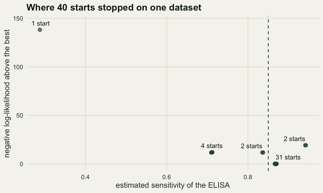
The 40 random starts stopped at 5 distinct places. 9 of them, 22 per cent, stopped more than one unit of negative log-likelihood above the best, and all 4 inferior stopping places have at least one parameter pinned at zero or one: a specificity of one, or a prevalence of zero in the newer district. The start with the newer district’s prevalence at 0.6 stopped 19.2 units of negative log-likelihood above the best. Those are not small differences in a flat region. A likelihood ratio of that size would be decisive evidence if it were a comparison between models, and here it is the same model with a different start.
The label swap from the occupancy post also exists here: replacing each prevalence with one minus itself, and swapping each sensitivity with one minus the matching specificity, gives the same likelihood. It was not a problem in these runs, because random starts with accuracies above 0.5 never crossed to the mirror solution; the fits keep the labelling in which a positive result makes infection more likely. The simulation code below still discards any fit with sensitivity plus specificity below one, as a guard; it almost never had anything to discard.
The best optimum is often on the boundary, as predicted
A single dataset is an anecdote. The simulation below draws 300 pairs of districts for each combination of prevalence gap and sample size, fits each from the default start and from 10 random starts, and treats the best of those 11 fits as the maximum likelihood estimate. For each dataset it records whether the default start, and what share of the single random starts, stopped more than one unit of negative log-likelihood above that best fit, whether the best fit has any parameter within 0.001 of zero or one, and whether the ELISA’s estimated sensitivity is itself at one. It also computes the Wald interval on the logit scale from the numerical Hessian, and the profile likelihood interval for the ELISA’s sensitivity and the older district’s prevalence, checked by asking whether the profile deviance at the true value is below the chi squared cut-off. The profile at a sensitivity of 0.99 is recorded too; if that value is inside the interval, the data have not bounded sensitivity from above.
analyse_one <- function(y1, y2, prev2, truth_start) {
  fit_def <- hw_fit(start_default, y1, y2)
  fits <- cbind(fit_def, sapply(seq_len(n_rand), function(i) hw_fit(start_random(), y1, y2)))
  fits <- fits[, fits[3, ] + fits[5, ] >= 1, drop = FALSE]
  best <- fits[, which.min(fits["nll", ])]
  near <- pmin(pmax(best[1:6], 0.02), 0.98)
  prof <- function(j, value) {
    2 * (min(hw_fit(near, y1, y2, j, value), hw_fit(truth_start, y1, y2, j, value)) - best[["nll"]])
  }
  hess <- tryCatch(optimHess(qlogis(best[1:6]), hw_nll, hw_grad, y1 = y1, y2 = y2),
                   error = function(e) NULL)
  vcov_hat <- tryCatch(solve(hess), error = function(e) NULL)
  wald_cover <- function(j, truth) {
    if (is.null(vcov_hat) || !is.finite(vcov_hat[j, j]) || vcov_hat[j, j] <= 0) return(NA)
    abs(qlogis(truth) - qlogis(best[[j]])) < qnorm(0.975) * sqrt(vcov_hat[j, j])
  }
  c(default_miss = fit_def[["nll"]] - best[["nll"]] > miss_tol,
    default_excess = fit_def[["nll"]] - best[["nll"]],
    random_miss = mean(fits["nll", -1] - best[["nll"]] > miss_tol),
    boundary = any(best[1:6] > 0.999 | best[1:6] < 0.001),
    se1_one = best[[3]] > 0.999, sp2_one = best[[6]] > 0.999,
    se1_hat = best[[3]], prev1_hat = best[[1]],
    wald_se1 = wald_cover(3, se_true[1]), wald_prev1 = wald_cover(1, prev1),
    prof_se1 = prof(3, se_true[1]) < crit, prof_prev1 = prof(1, prev1) < crit,
    open_se1 = prof(3, 0.99) < crit)
}
run_cell <- function(prev2, n, cov_pos = 0, cov_neg = 0) {
  pr1 <- cell_prob(prev1, se_true[1], se_true[2], sp_true[1], sp_true[2], cov_pos, cov_neg)
  pr2 <- cell_prob(prev2, se_true[1], se_true[2], sp_true[1], sp_true[2], cov_pos, cov_neg)
  truth_start <- c(prev1, prev2, se_true, sp_true)
  t(replicate(n_rep, analyse_one(rmultinom(1, n, pr1)[, 1], rmultinom(1, n, pr2)[, 1],
                                 prev2, truth_start)))
}
set.seed(2024)
grid_cells <- expand.grid(prev2 = prev2_set, n = n_set)
grid_raw <- lapply(seq_len(nrow(grid_cells)), function(i) run_cell(grid_cells$prev2[i], grid_cells$n[i]))
grid_sum <- cbind(grid_cells, gap = prev1 - grid_cells$prev2,
                  t(sapply(grid_raw, function(m) colMeans(m, na.rm = TRUE))),
                  wald_na = sapply(grid_raw, function(m) mean(is.na(m[, "wald_se1"]))))
gcell <- function(gap, n) grid_sum[abs(grid_sum$gap - gap) < 1e-9 & grid_sum$n == n, ]
mcse_max <- sqrt(0.25 / n_rep)
mcse_cov <- sqrt(0.95 * 0.05 / n_rep)
round(grid_sum[, c("gap", "n", "default_miss", "random_miss", "boundary", "se1_one", "open_se1")], 3)
gap n default_miss random_miss boundary se1_one open_se1
1 0.05 200 0.00 0.006 0.743 0.250 0.990
2 0.10 200 0.00 0.009 0.687 0.213 0.937
3 0.25 200 0.00 0.081 0.167 0.053 0.637
4 0.05 800 0.00 0.013 0.583 0.180 0.943
5 0.10 800 0.00 0.021 0.453 0.060 0.707
6 0.25 800 0.01 0.210 0.003 0.000 0.097With 300 datasets per cell, a share has a Monte Carlo standard error of at most 0.029.
The default start is safe. In the worst cell it stopped more than one unit above the best fit in 1.0 per cent of datasets. A random start is less safe, and the false optima of the previous section belong to the well identified case: at a gap of 0.25 a single random start misses the best fit in 8.1 per cent of datasets with 200 animals and 21.0 per cent with 800, against 0.6 and 1.3 per cent at a gap of 0.05. Ten starts and a comparison of their log-likelihoods is cheap insurance, and a start with the prevalences the wrong way round, as in the single dataset above, is the kind to avoid.
Starts do not cure the boundary. With a gap of 0.10 and 200 animals per district, the best fit has a parameter at zero or one in 68.7 per cent of datasets, the ELISA’s sensitivity is estimated at exactly one in 21.3 per cent, and the profile interval for that sensitivity reaches 0.99 in 93.7 per cent. Part of that share is the rapid test’s specificity, estimated at one in 30.3 per cent of datasets; its true value is 0.98, so that boundary is a small error. A sensitivity of one for a test whose true sensitivity is 0.85 is not. Four times as many animals help less than one might hope: at a gap of 0.10 and 800 animals the boundary share is 45.3 per cent and the sensitivity is still unbounded above in 70.7 per cent. Only the combination of a gap of 0.25 and 800 animals makes the boundary rare, at 0.3 per cent, with the sensitivity interval open to 0.99 in 9.7 per cent of datasets.
This is what Hui and Walter’s condition of different prevalences looks like at a finite sample. The model is identified as soon as the prevalences differ and neither test is a coin toss (sensitivity plus specificity above one), but the information about the accuracies comes from the difference, and a difference of 0.10 between two samples of 200 is not much of one. That information can be computed before any data exist. The chunk below builds the expected Fisher information of the model at the design values, from the derivatives of the eight cell probabilities, inverts it for the asymptotic standard error of the ELISA’s sensitivity, and turns it into a normal approximation to the chance that the estimate reaches one.
info_se <- function(prev2, n, h = 1e-6) {
  par0 <- c(prev1, prev2, se_true, sp_true)
  cells <- function(par) c(cell_prob(par[1], par[3], par[4], par[5], par[6]),
                           cell_prob(par[2], par[3], par[4], par[5], par[6]))
  jac <- sapply(1:6, function(j) {
    e <- replace(numeric(6), j, h)
    (cells(par0 + e) - cells(par0 - e)) / (2 * h)
  })
  fisher <- n * t(jac) %*% diag(1 / cells(par0)) %*% jac
  sqrt(diag(solve(fisher)))
}
bnd_pred <- data.frame(gap = grid_sum$gap, n = grid_sum$n,
  se_se1 = mapply(function(p2, nn) info_se(p2, nn)[3], grid_sum$prev2, grid_sum$n))
bnd_pred$predicted <- 1 - pnorm((1 - se_true[1]) / bnd_pred$se_se1)
bnd_pred$simulated <- grid_sum$se1_one
bnd_pred$sim_sd <- sapply(grid_raw, function(m) sd(m[, "se1_hat"]))
pcell <- function(gap, n) bnd_pred[abs(bnd_pred$gap - gap) < 1e-9 & bnd_pred$n == n, ]
round(bnd_pred, 3)
gap n se_se1 predicted simulated sim_sd
1 0.05 200 0.373 0.344 0.250 0.093
2 0.10 200 0.189 0.213 0.213 0.093
3 0.25 200 0.079 0.029 0.053 0.079
4 0.05 800 0.186 0.210 0.180 0.085
5 0.10 800 0.094 0.056 0.060 0.073
6 0.25 800 0.040 0.000 0.000 0.039At a gap of 0.10 with 200 animals the asymptotic standard error of the sensitivity is 0.189, and the predicted share of estimates at one is 0.213 against 0.213 simulated. With 800 animals the prediction is 0.056 and the simulation 0.060; at a gap of 0.05 and 800 animals, 0.210 and 0.180. The approximation breaks where the standard error is large enough that a normal distribution is a poor description of an estimate confined to the unit interval: at a gap of 0.05 with 200 animals it predicts 0.344 and the simulation gives 0.250. So the boundary share is not a finding of the simulation. It is the weak identifiability of the model at a small prevalence gap, and anyone planning a study can compute it from the design values in a second.
The prevalence difference is one of the assumptions Toft, Jorgensen and Hojsgaard (2005) say have to be checked before the estimates mean anything. They list it with two others: conditional independence, which the last section takes up, and accuracies that are the same in both populations. The second is the fragile one in this scenario, because a district where the virus arrived last winter has a larger share of recent, low-titre infections, and an antibody test is less sensitive in exactly that district. The model has one sensitivity per test for both districts, so it cannot notice.
bnd_long <- do.call(rbind, lapply(c("random_miss", "boundary", "se1_one", "open_se1"), function(v)
  data.frame(gap = grid_sum$gap, n = paste(grid_sum$n, "animals per district"),
             measure = v, share = grid_sum[[v]])))
bnd_long$measure <- factor(bnd_long$measure,
  levels = c("open_se1", "boundary", "se1_one", "random_miss"),
  labels = c("profile interval reaches 0.99", "any parameter at 0 or 1",
             "ELISA sensitivity at 1", "one random start misses best"))
ggplot(bnd_long, aes(gap, share, colour = measure)) +
  geom_line(linewidth = 0.9) + geom_point(size = 2.2) +
  facet_wrap(~ n) +
  scale_colour_manual(values = c(te_ink, te_forest, te_gold, te_rust), name = NULL) +
  scale_x_continuous(breaks = prev1 - prev2_set) +
  scale_y_continuous(limits = c(0, 1)) +
  labs(x = "difference in prevalence between districts", y = "share of datasets",
       title = "A small prevalence gap leaves the estimate unbounded") +
  theme_datasheet() +
  theme(legend.position = "bottom") +
  guides(colour = guide_legend(nrow = 2))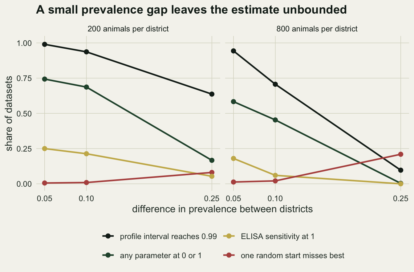
Wald and profile intervals fail in opposite directions
cov_long <- do.call(rbind, lapply(c("wald_se1", "prof_se1", "wald_prev1", "prof_prev1"), function(v)
  data.frame(gap = grid_sum$gap, n = factor(grid_sum$n), var = v, coverage = grid_sum[[v]])))
cov_long$method <- ifelse(grepl("^wald", cov_long$var), "Wald, logit scale", "profile likelihood")
cov_long$parameter <- ifelse(grepl("se1", cov_long$var), "ELISA sensitivity", "prevalence, older district")
ggplot(cov_long, aes(gap, coverage, colour = method, linetype = n)) +
  geom_hline(yintercept = 0.95, linetype = "dashed", colour = te_body) +
  geom_line(linewidth = 0.9) + geom_point(size = 2) +
  facet_wrap(~ parameter) +
  scale_colour_manual(values = c(te_forest, te_rust), name = NULL) +
  scale_linetype_manual(values = c("dotted", "solid"), name = "animals per district") +
  scale_x_continuous(breaks = prev1 - prev2_set) +
  labs(x = "difference in prevalence between districts", y = "coverage",
       title = "Coverage of 95 per cent intervals") +
  theme_datasheet() +
  theme(legend.position = "bottom", legend.box = "vertical")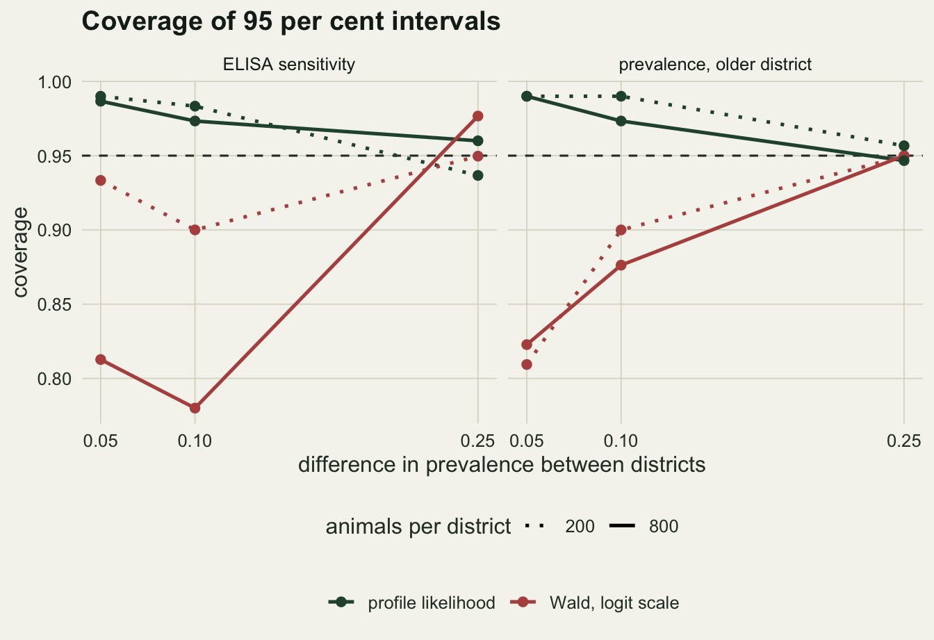
The two interval methods fail in opposite directions. The Wald interval, built on the logit scale from the curvature at the best fit, undercovers at gaps of 0.05 and 0.10, where its coverage runs from 0.780 to 0.933. For the sensitivity more animals make it worse rather than better: at a gap of 0.10 its coverage of the ELISA’s sensitivity is 0.900 with 200 animals per district and 0.780 with 800. For the older district’s prevalence at a gap of 0.05 the extra animals barely move it: 0.809 and 0.823.
wald_split <- data.frame(gap = grid_sum$gap, n = grid_sum$n, t(sapply(grid_raw, function(m) {
  at_one <- m[, "se1_one"] == 1
  c(n_at_one = sum(at_one), covered_at_one = sum(m[at_one, "wald_se1"], na.rm = TRUE),
    interior_cover = mean(m[!at_one, "wald_se1"], na.rm = TRUE))
})))
wcell <- function(gap, n) wald_split[abs(wald_split$gap - gap) < 1e-9 & wald_split$n == n, ]
n_wald_low <- sum(unlist(grid_sum[grid_sum$gap < 0.2, c("wald_se1", "wald_prev1")]) < 0.95 - 2 * mcse_cov)
round(wald_split, 3)
gap n n_at_one covered_at_one interior_cover
1 0.05 200 75 75 0.911
2 0.10 200 64 64 0.873
3 0.25 200 16 16 0.947
4 0.05 800 54 54 0.771
5 0.10 800 18 18 0.766
6 0.25 800 0 0 0.977The boundary is not where the Wald interval fails. Splitting the datasets by whether the sensitivity was estimated at one shows that those fits are always covered: 227 of 227 across the grid, because the logit-scale standard error at an estimate of one is enormous. The shortfall comes entirely from interior fits, whose Wald coverage of the sensitivity is 0.771 and 0.766 with 800 animals at gaps of 0.05 and 0.10. Away from a gap of 0.25 the log-likelihood is far from quadratic even on the logit scale, and an interior estimate with a moderate curvature at its peak gets an interval that is too short on the side where the likelihood stays flat. Two things push the sensitivity coverage down as animals are added: at a gap of 0.10 the interior coverage itself falls from 0.873 with 200 animals to 0.766 with 800, and the always-covered fits at one shrink from 64 to 18 of 300. With 300 datasets per cell, a coverage has a Monte Carlo standard error of 0.013, and 7 of the eight Wald coverages at gaps of 0.05 and 0.10 are more than two Monte Carlo standard errors below 0.95; the exception is the sensitivity at a gap of 0.05 with 200 animals, at 0.933.
The profile interval keeps its coverage in every cell of the grid, between 0.937 and 0.990, and at small gaps it does so by being uninformative. When the interval for sensitivity reaches 0.99 in 99.0 per cent of datasets, as at a gap of 0.05 with 200 animals, covering 0.85 is not an achievement. So the answer to whether profile intervals hold their level at 200 animals with a small gap is yes, and the interval is the honest report: it says the data do not bound the sensitivity. Only at a gap of 0.25 are both methods within 0.027 of 0.95, where the Monte Carlo standard error of a coverage near 0.95 is 0.013.
Dependence the fit cannot see
Two assays that detect the same antibody tend to miss the same animals: an early infection with a low titre is negative on both. That is a positive conditional covariance among infected animals, the cov_pos argument of cell_prob. The model has no parameter for it and no spare degrees of freedom to estimate one. What the fit does with dependent data can be computed without simulation, by fitting the model to the expected counts, which is where the estimate settles as the sample grows.
cov_pos_max <- min(se_true[1] * (1 - se_true[2]), (1 - se_true[1]) * se_true[2])
cov_neg_max <- min((1 - sp_true[1]) * sp_true[2], sp_true[1] * (1 - sp_true[2]))
sd_inf   <- sqrt(se_true[1] * (1 - se_true[1]) * se_true[2] * (1 - se_true[2]))
sd_uninf <- sqrt(sp_true[1] * (1 - sp_true[1]) * sp_true[2] * (1 - sp_true[2]))
limit_fit <- function(prev2, cov_pos, cov_neg = 0) {
  e1 <- 800 * cell_prob(prev1, se_true[1], se_true[2], sp_true[1], sp_true[2], cov_pos, cov_neg)
  e2 <- 800 * cell_prob(prev2, se_true[1], se_true[2], sp_true[1], sp_true[2], cov_pos, cov_neg)
  fits <- cbind(hw_fit(start_default, e1, e2), hw_fit(c(prev1, prev2, se_true, sp_true), e1, e2),
                sapply(1:n_rand, function(i) hw_fit(start_random(), e1, e2)))
  fits <- fits[, fits[3, ] + fits[5, ] >= 1, drop = FALSE]
  best <- fits[, which.min(fits["nll", ])]
  gap_fit <- max(abs(cell_prob(best[1], best[3], best[4], best[5], best[6]) - e1 / 800))
  c(se1 = best[[3]], prev1 = best[[1]], prev2 = best[[2]], fit_gap = gap_fit)
}
set.seed(515)
cov_pos_grid <- seq(0, 0.10, by = 0.01)
lim_pos <- as.data.frame(t(sapply(cov_pos_grid, function(cv) limit_fit(0.05, cv))))
lim_pos$cov <- cov_pos_grid
cov_neg_grid <- c(0, 0.005, 0.01, 0.015)
lim_neg <- as.data.frame(t(sapply(cov_neg_grid, function(cv) limit_fit(0.05, 0, cv))))
lim_neg$cov <- cov_neg_grid

set.seed(909)
dep_cells <- expand.grid(cov_pos = c(0.02, 0.05), n = n_set)
dep_raw <- lapply(seq_len(nrow(dep_cells)), function(i) run_cell(0.05, dep_cells$n[i], dep_cells$cov_pos[i]))
dep_sum <- cbind(dep_cells,
  se1_med   = sapply(dep_raw, function(m) median(m[, "se1_hat"])),
  prev1_med = sapply(dep_raw, function(m) median(m[, "prev1_hat"])),
  off_share = sapply(dep_raw, function(m) mean(abs(m[, "se1_hat"] - se_true[1]) > 0.10)),
  prof_se1  = sapply(dep_raw, function(m) mean(m[, "prof_se1"])),
  prof_prev1 = sapply(dep_raw, function(m) mean(m[, "prof_prev1"])),
  wald_prev1 = sapply(dep_raw, function(m) mean(m[, "wald_prev1"], na.rm = TRUE)))
dep_sum$lim_se1   <- sapply(dep_sum$cov_pos, function(cv) lim_pos$se1[abs(lim_pos$cov - cv) < 1e-9])
dep_sum$lim_prev1 <- sapply(dep_sum$cov_pos, function(cv) lim_pos$prev1[abs(lim_pos$cov - cv) < 1e-9])
dcell <- function(cv, n) dep_sum[abs(dep_sum$cov_pos - cv) < 1e-9 & dep_sum$n == n, ]
round(dep_sum, 3)
cov_pos n se1_med prev1_med off_share prof_se1 prof_prev1 wald_prev1
1 0.02 200 0.881 0.289 0.213 0.950 0.930 0.929
2 0.05 200 0.923 0.274 0.343 0.867 0.927 0.946
3 0.02 800 0.871 0.293 0.033 0.890 0.943 0.957
4 0.05 800 0.917 0.275 0.193 0.550 0.837 0.873
lim_se1 lim_prev1
1 0.877 0.290
2 0.918 0.276
3 0.877 0.290
4 0.918 0.276The largest covariance among infected animals that these sensitivities allow is 0.1125, so 0.02 and 0.05 are correlations between the two test results among infected animals of 0.13 and 0.32. The simulation sets the newer district’s prevalence at 0.05, a gap of 0.25, the design where independent tests gave well determined estimates with 800 animals per district (with 200 the sensitivity interval was still open to 0.99 in 63.7 per cent of datasets).
As the sample grows, a covariance of 0.02 moves the ELISA’s estimated sensitivity from 0.85 to 0.877 and the older district’s prevalence from 0.30 to 0.290. A covariance of 0.05 gives 0.918 and 0.276, and 0.10 gives 0.987 and 0.256. At every covariance on the grid the fitted cell probabilities match the expected ones to within 5.86e-07: the model fits dependent data perfectly, so no test on the fit can reveal the dependence. The direction is the one Vacek (1985) derived and the one the capture-recapture model Mh has: animals that both tests miss are invisible to both, so the infected class shrinks and the tests look more sensitive than they are. Dependence among uninfected animals acts on prevalence the other way; a covariance of 0.015 there leaves the sensitivity at 0.850 and raises the older district’s prevalence to 0.318.
The simulated medians sit on the limiting values: with 800 animals and a covariance of 0.05 the median sensitivity is 0.917 against a limit of 0.918. The bias is arithmetic, and it can be computed for any assumed covariance before a study starts. What that arithmetic does not show is what happens to the interval. With 800 animals and a covariance of 0.05 the profile interval covers the true sensitivity in 0.550 of datasets and the true prevalence in 0.837; at a covariance of 0.02 the figures are 0.890 and 0.943. With 200 animals the same shift hides inside wider intervals, and sensitivity coverage is 0.950 and 0.867 at the two covariances. More animals make the interval tighter around the wrong value. The share of datasets with the sensitivity more than 0.10 from the truth, on the other hand, is larger with fewer animals: 0.343 at 200 and 0.193 at 800 for a covariance of 0.05, because at 200 animals sampling error adds to the bias.
sim_pts <- rbind(data.frame(cov = dep_sum$cov_pos, value = dep_sum$se1_med, n = factor(dep_sum$n), what = "ELISA sensitivity"),
                 data.frame(cov = dep_sum$cov_pos, value = dep_sum$prev1_med, n = factor(dep_sum$n), what = "prevalence, older district"))
base_pts <- rbind(data.frame(cov = 0, value = sapply(n_set, function(nn) median(grid_raw[[which(grid_cells$prev2 == 0.05 & grid_cells$n == nn)]][, "se1_hat"])),
                             n = factor(n_set), what = "ELISA sensitivity"),
                  data.frame(cov = 0, value = sapply(n_set, function(nn) median(grid_raw[[which(grid_cells$prev2 == 0.05 & grid_cells$n == nn)]][, "prev1_hat"])),
                             n = factor(n_set), what = "prevalence, older district"))
lim_long <- rbind(data.frame(cov = lim_pos$cov, value = lim_pos$se1, what = "ELISA sensitivity"),
                  data.frame(cov = lim_pos$cov, value = lim_pos$prev1, what = "prevalence, older district"))
truth_df <- data.frame(what = c("ELISA sensitivity", "prevalence, older district"), value = c(se_true[1], prev1))
ggplot(lim_long, aes(cov, value)) +
  geom_hline(data = truth_df, aes(yintercept = value), linetype = "dashed", colour = te_body) +
  geom_line(colour = te_forest, linewidth = 1) +
  geom_point(data = rbind(sim_pts, base_pts), aes(shape = n), colour = te_rust, size = 2.6) +
  facet_wrap(~ what, scales = "free_y") +
  scale_shape_manual(values = c(1, 16), name = "animals per district") +
  labs(x = "conditional covariance between tests among infected animals", y = "estimate",
       title = "Dependence moves the estimate, and the fit stays perfect") +
  theme_datasheet() +
  theme(legend.position = "bottom")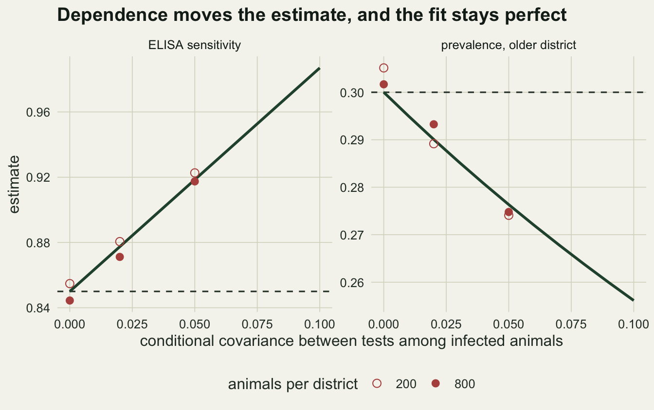
What to report
Give the two-by-two table of test results for each population. It is eight numbers, the model is saturated, and with them any reader can refit the model under a different assumption.
Give the prevalence difference between the populations and treat it as a design quantity. The simulations here suggest that a difference of 0.10 with a few hundred animals per population leaves the accuracies weakly determined whatever the software, and that is worth knowing before the samples are drawn rather than after. The info_se function above gives a first check for a planned design: with the design values set to the expected prevalence of the first population and the expected accuracies, give it the second prevalence and the number of animals, and it returns the asymptotic standard error of each parameter. Read a large value as a warning, not as the spread to expect: at a gap of 0.10 with 200 animals it is 0.189 for the ELISA’s sensitivity, while the simulated estimates, piled against one, have a standard deviation of 0.093.
Say how many starts were used and whether their log-likelihoods agreed. If some runs stopped at a different optimum, give its log-likelihood and the estimates there; a false optimum with a specificity of one or a prevalence of zero is a result an unwary analysis would publish.
Report any estimate at zero or one as a boundary estimate, and use profile likelihood intervals. If the interval for a sensitivity or specificity runs to the upper limit, say that the data do not bound it from above. That sentence is more useful to the next study than a Wald interval that looks narrow.
State the conditional independence assumption in biological terms and argue it. Two assays that detect the same antibody are the case where dependence among infected animals should be expected; an antibody test paired with a test for the agent itself is a better argument for independence. Argue the same way that the accuracies are the same in both populations: if one population is at an earlier stage of the epidemic, or is a different age mix, an antibody test’s sensitivity is unlikely to be. Where dependence is plausible, fit the model to expected counts under an assumed covariance, as in the limit_fit function above, and report how far the estimates move.
Honest limits
One set of accuracies and one prevalence in the older district were simulated, both fixed before the runs. A pair of tests with lower specificity, or populations with prevalences nearer one half, would give different boundary rates, and the numbers here are not design advice for another pair of tests without rerunning the code. The rapid test’s true specificity of 0.98 is close to one, which inflates the share of fits with a parameter at the boundary; the ELISA sensitivity at one is the cleaner measure of the problem.
The best of eleven starts is treated as the maximum likelihood estimate. That is a practical definition, not a proof, and a few datasets may have a better optimum that no start reached. The profile deviance at the true value was minimised from two starts, one of them the truth itself; that is a simulation convenience for checking coverage, and an analyst without the truth finds the interval endpoints by searching along the profile instead.
Everything here is maximum likelihood. Many applied Hui-Walter analyses in veterinary epidemiology are Bayesian, with informative priors on at least some accuracies. A prior that keeps a sensitivity away from one removes the boundary estimate, but it does so by supplying information the two tables do not contain, and with vague priors the posterior can be expected to put mass near one wherever the profile interval is open. That comparison was not run.
Accuracies were the same in both districts in every simulation. If the ELISA is less sensitive in the newer district, the model has no parameter for the difference either, and what that does to the estimates and intervals was not simulated here.
Dependence was simulated as a single fixed covariance among infected animals, and among uninfected animals only through the limiting fit. In real serology the dependence varies with the stage of infection and the antibody titre, which is a mixture the covariance summarises but does not describe. Georgiadis, Johnson, Gardner and Singh (2003) add covariance parameters to the model. With two populations the tables have no degrees of freedom to spare for them, so the information has to come from more populations or from priors.
References
Hui SL, Walter SD 1980 Biometrics 36(1):167-171 (10.2307/2530508)
Vacek PM 1985 Biometrics 41(4):959-968 (10.2307/2530967)
Georgiadis MP, Johnson WO, Gardner IA, Singh R 2003 Journal of the Royal Statistical Society Series C 52(1):63-76 (10.1111/1467-9876.00389)
Toft N, Jorgensen E, Hojsgaard S 2005 Preventive Veterinary Medicine 68(1):19-33 (10.1016/j.prevetmed.2005.01.006)