Digit preference and heaping in field data

Recorders drift towards round numbers and the mean drifts with them. Measuring digit heaping in R: the Whipple index, the bias it hides, and a mixture repair.

An upland river carries a restoration scheme: two hundred metres of channel where large wood was reinstated four years ago, and a control reach two kilometres downstream that was left as it was. Both are electrofished on the same September day, three passes each, and in a decent year about six hundred young trout come out of each reach. Every fish goes onto a measuring board, fork length read to the nearest millimetre, called out and written on a waterproof sheet. The restored reach is nearest the gate, so it is always fished first. The control reach is done last, in poor light, by people who have been standing in cold water since eight in the morning.

The board reads to the millimetre all day. The sheet does not. A fish that measures 83 in the morning is written 83; the same fish at half past five is written 80, because the observer’s eye goes to the labelled centimetre mark and the difference does not feel worth the argument. Some fish get 85 instead. Almost none get 82 or 87. The recorded lengths pile up on the digits 0 and 5, they pile up harder on 0 than on 5, and they pile up asymmetrically, because a fish just over a round number is written at that round number more often than a fish just under it is pushed up to the next one.

That last clause is the whole post. Rounded and coarsened measurements took the other case: a known regular grid applied to every observation, where the recorded value is a deterministic function of the true one. There the mean survived intact, the variance gained a predictable amount, the distributional tests rejected the ruler rather than the biology, and an interval-censored likelihood put everything back. Heaping is not that. It is behaviour rather than arithmetic, it has a direction, and the mean does not survive it.

Two posts on the site already say so in passing without a number attached. Distance sampling for density in R lists heaping at round numbers among the things that distort the histogram near the line, and checking a distance sampling model puts “no heaping on round numbers” in its table of assumptions. This post supplies the measurement behind that mention; Marques (2004) is the distance-specific treatment, where the resolution scales with the distance itself.

Four things get measured. Whether heaping can be detected from the recorded numbers alone, and how much of it a scheme of a given size can see. How large the bias in the mean is, and where it comes from. What differential heaping does to a comparison between two arms with no true difference between them. And how much of the damage a mixture model can undo before the mechanism stops being ignorable.

library(ggplot2)

te_pal <- list(forest = "#275139", green = "#2f8f63", sage = "#93a87f",
               clay = "#b5534e", gold = "#cda23f", line = "#dad9ca",
               ink = "#16241d", paper = "#f5f4ee")

theme_te <- function() {
  theme_minimal(base_size = 12) +
    theme(panel.grid.minor = element_blank(),
          panel.grid.major = element_line(colour = "#e7e6dc"),
          plot.background = element_rect(fill = "#f5f4ee", colour = NA),
          panel.background = element_rect(fill = "#f5f4ee", colour = NA),
          plot.title = element_text(face = "bold", colour = te_pal$ink),
          axis.title = element_text(colour = "#2c3a31"),
          axis.text = element_text(colour = "#2c3a31"),
          legend.position = "bottom")
}

A model of the recorder

The mechanism has to be explicit before anything can be measured against it, and the version below is deliberately the simplest one that keeps the two features the field sheet shows. Multiples of ten attract more strongly than the odd multiples of five, and the pull is asymmetric.

Each fish is measured to the millimetre. With probability p10 the recorder writes the nearest multiple of ten instead, choosing the one below with probability one plus the asymmetry over two and the one above otherwise. Failing that, with probability p5 the same happens with multiples of five. A reading that already sits on the attractor stays where it is. An asymmetry of zero means a recorder who is careless but even handed; an asymmetry of one means a recorder who never rounds upwards.

heap_record <- function(x, p10, p5, asym) {
  n <- length(x)
  fine <- round(x)
  y <- fine
  u <- runif(n)
  down <- runif(n) < (1 + asym) / 2
  hit10 <- u < p10
  hit5 <- (!hit10) & (u < p10 + (1 - p10) * p5)
  r10 <- fine %% 10
  r5 <- fine %% 5
  m10 <- hit10 & r10 != 0
  m5 <- hit5 & r5 != 0
  y[m10] <- ifelse(down[m10], fine[m10] - r10[m10], fine[m10] + 10 - r10[m10])
  y[m5] <- ifelse(down[m5], fine[m5] - r5[m5], fine[m5] + 5 - r5[m5])
  y
}

mu_fish <- 78
sd_fish <- 11
n_reach <- 600
crew_am <- c(p10 = 0.10, p5 = 0.10, asym = 0.20)
crew_pm <- c(p10 = 0.45, p5 = 0.35, asym = 0.80)

set.seed(20260801)
peek <- rnorm(12, mu_fish, sd_fish)
demo <- data.frame(
  board = round(peek),
  morning = heap_record(peek, crew_am[1], crew_am[2], crew_am[3]),
  afternoon = heap_record(peek, crew_pm[1], crew_pm[2], crew_pm[3]))
print(demo)

   board morning afternoon
1     59      59        59
2     78      78        70
3     81      81        80
4     63      63        63
5     45      45        40
6     83      83        83
7     96      95        96
8     60      60        60
9     78      80        78
10    74      74        70
11    89      89        89
12    77      77        77

print(colSums(demo) - sum(demo$board))

    board   morning afternoon 
        0         1       -18 

Two properties of that map matter later and neither holds for a uniform grid. The move is random rather than deterministic, so the same fish measured twice can be written down two ways. And the two directions are not equally likely, so the errors do not cancel.

The mean shift follows from counting. Given that a reading is pulled to a multiple of ten, the remainder it has to travel is uniform on one to nine in either direction, an average of five millimetres, and the down and up probabilities differ by the asymmetry. Nine tenths of readings have a non-zero remainder. The expected shift from the ten tier is therefore minus four and a half times p10 times the asymmetry, and the five tier contributes its own term on the same pattern.

The terminal digit is the only witness

Nothing in a column of fork lengths says who measured them or when. The one thing the column does carry is its own last digit, and under any reasonable population that digit should be uniform. That statement sounds like an assumption about the biology and is not. The distribution of the last digit is the latent density aliased onto a cycle of ten, so its departure from uniform is governed by the density’s Fourier coefficient at that frequency, which for anything smooth on a ten millimetre scale is negligible.

digit_probs <- function(mu, s) {
  v <- seq(round(mu - 12 * s), round(mu + 12 * s))
  pr <- pnorm(v + 0.5, mu, s) - pnorm(v - 0.5, mu, s)
  as.numeric(tapply(pr, v %% 10, sum))
}

dp_wide <- max(abs(digit_probs(mu_fish, sd_fish) - 0.1))
dp_mid <- max(abs(digit_probs(mu_fish, 4) - 0.1))
dp_narrow <- max(abs(digit_probs(mu_fish, 2) - 0.1))
print(signif(c(sd_11mm = dp_wide, sd_4mm = dp_mid, sd_2mm = dp_narrow), 4))

  sd_11mm    sd_4mm    sd_2mm 
8.337e-12 8.361e-03 9.741e-02 

With a standard deviation of 11 millimetres the largest departure of any digit probability from a tenth is 8.34e-12, which is not a rounding error in the argument but an exact calculation from pnorm. Squeeze the population down to a standard deviation of 4 mm and it is still only 0.00836. At 2 mm, narrower than the digit cycle itself, it reaches 0.0974 and the null stops being safe. For a length-frequency sample that spans several centimetres the uniform digit null is exact for practical purposes, which is what makes the terminal digit a usable instrument.

The classic summary of that digit table is the Whipple index, built a century ago for age heaping in census returns and still the standard instrument in that literature (A’Hearn, Baten and Crayen 2009): the share of values ending in 0 or 5, divided by the fifth that uniformity predicts, multiplied by a hundred. Roberts and Brewer (2001) set out the family it belongs to and what each member is sensitive to. It is two lines of base R.

whipple <- function(y) 500 * mean((y %% 10) %in% c(0, 5))

set.seed(20260802)
n_null <- c(100, 250, 600, 1500)
null_res <- do.call(rbind, lapply(n_null, function(nn) {
  wv <- replicate(4000, whipple(round(rnorm(nn, mu_fish, sd_fish))))
  data.frame(n = nn, mean_w = mean(wv), sd_w = sd(wv),
             analytic_sd = 200 / sqrt(nn),
             q95 = unname(quantile(wv, 0.95)))
}))
print(round(null_res, 3))

     n  mean_w   sd_w analytic_sd     q95
1  100  99.488 19.919      20.000 135.000
2  250  99.830 12.699      12.649 122.000
3  600  99.824  8.055       8.165 113.333
4 1500 100.055  5.074       5.164 108.333

w_crit <- null_res$q95[null_res$n == n_reach]

The index sits on 99.82 when nothing is wrong, and its sampling standard deviation is exactly the binomial one: the count of values ending in 0 or 5 is a draw from a binomial with probability a fifth, so the index has standard deviation two hundred over the square root of n. The simulated and analytic values agree across the table, 8.06 against 8.16 at six hundred fish. A reach of that size gives a one-sided five per cent threshold of 113.3. Anything below that is noise, and quoting an index of 108 from a sample of a hundred, which happens, is quoting noise.

Now the three ways the same six hundred fish could reach the spreadsheet: read to the millimetre, read onto a uniform five millimetre grid in the manner of the companion post, and read by the afternoon crew.

round_to <- function(x, h) h * round(x / h)

set.seed(20260803)
z_reach <- rnorm(n_reach, mu_fish, sd_fish)
y_fine <- round(z_reach)
y_grid <- round_to(z_reach, 5)
y_heap <- heap_record(z_reach, crew_pm[1], crew_pm[2], crew_pm[3])

digit_tab <- function(y) as.integer(table(factor(y %% 10, levels = 0:9)))
digit_p <- function(y) suppressWarnings(chisq.test(digit_tab(y))$p.value)

three <- data.frame(
  column = c("fine", "uniform 5 mm grid", "afternoon crew"),
  whipple = c(whipple(y_fine), whipple(y_grid), whipple(y_heap)),
  chisq_p = c(digit_p(y_fine), digit_p(y_grid), digit_p(y_heap)),
  mean_mm = c(mean(y_fine), mean(y_grid), mean(y_heap)))
print(three, digits = 5)

             column whipple     chisq_p mean_mm
1              fine   87.50  9.2784e-02  78.450
2 uniform 5 mm grid  500.00  0.0000e+00  78.575
3    afternoon crew  354.17 3.2114e-322  76.757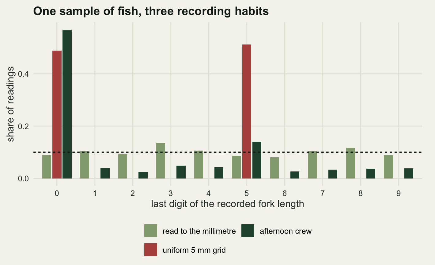

Figure 1: Distribution of the last digit of the recorded fork length for six hundred young trout, the same fish written down three ways. Read to the millimetre the ten digits are level. Read onto a uniform five millimetre grid all the mass sits on 0 and 5. Read by a crew that drifts towards round numbers the profile is intermediate, with a tall bar at 0, a shorter one at 5 and the eight other digits depleted.

The millimetre column returns an index of 87.5, under the threshold of 113.3 and so not evidence of anything. The uniform grid returns 500, the ceiling, because every value on a five millimetre grid ends in 0 or 5. The afternoon crew returns 354.2. The interesting question is how small a habit a reach of six hundred fish can still see, which needs the index turned into a test and run against a graded series of offenders.

set.seed(20260804)
p_seq <- c(0, 0.01, 0.02, 0.04, 0.06, 0.10, 0.15)
pow_res <- do.call(rbind, lapply(p_seq, function(pp) {
  M <- t(replicate(1200, {
    yy <- heap_record(rnorm(n_reach, mu_fish, sd_fish), pp, 0, 0.8)
    c(whipple(yy), digit_p(yy))
  }))
  data.frame(p10 = pp, whipple_pow = mean(M[, 1] > w_crit),
             chisq_pow = mean(M[, 2] < 0.05),
             mean_index = mean(M[, 1]))
}))
print(round(pow_res, 4))

   p10 whipple_pow chisq_pow mean_index
1 0.00      0.0500    0.0400   100.0271
2 0.01      0.1150    0.0608   103.9986
3 0.02      0.2450    0.1325   108.1146
4 0.04      0.5900    0.4900   115.7521
5 0.06      0.8783    0.8350   124.0118
6 0.10      0.9983    0.9983   139.5174
7 0.15      1.0000    1.0000   160.1312

pow_at <- function(pp) pow_res$whipple_pow[pow_res$p10 == pp]
chi_at <- function(pp) pow_res$chisq_pow[pow_res$p10 == pp]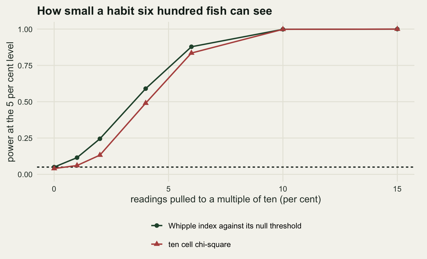

Figure 2: Power to detect heaping from the terminal digits of six hundred readings, as the share of readings pulled to a multiple of ten rises from none to fifteen per cent. The one degree of freedom Whipple test, comparing the index against its simulated null threshold, beats the ten cell chi-square at every heaping rate because it spends its power on the direction the heaping actually goes.

At two per cent of readings heaped the index has 24.5 per cent power and the omnibus chi-square 13.2 per cent. At four per cent the two are 59 and 49, and by six per cent both are near certainty. The gap is the cost of an omnibus test: the chi-square spreads nine degrees of freedom across all ten digits, while the index asks the single question the mechanism answers. Neither test needs anything except the column of numbers, which is the only good news in the post. Camarda, Eilers and Gampe (2008) go further and estimate the whole attraction pattern rather than a single index, which is the right tool when the attractor set is not known in advance.

The index sees the heaping and not the direction

Detection is the easy half. The index counts how many readings ended up on an attractor, and that count says nothing about which side they arrived from. Two recording habits with the same pull probability and opposite temperaments produce the same digit table.

set.seed(20260805)
z_pair <- rnorm(200000, mu_fish, sd_fish)
y_even <- heap_record(z_pair, 0.45, 0.35, 0)
y_down <- heap_record(z_pair, 0.45, 0.35, 0.8)

pair_tab <- rbind(even_handed = digit_tab(y_even), downward = digit_tab(y_down))
print(pair_tab)

              [,1] [,2] [,3] [,4] [,5]  [,6] [,7] [,8] [,9] [,10]
even_handed 116135 7285 7041 7141 7222 26517 7166 7082 7237  7174
downward    116029 7210 7070 7260 7168 26620 7192 7249 7078  7124

pair_test <- chisq.test(pair_tab)
pair_w <- c(even_handed = whipple(y_even), downward = whipple(y_down))
pair_mean <- c(board = mean(round(z_pair)), even_handed = mean(y_even),
               downward = mean(y_down))
print(round(c(pair_w, chisq = unname(pair_test$statistic),
              p = unname(pair_test$p.value)), 4))

even_handed    downward       chisq           p 
   356.6300    356.6225      5.8157      0.7582 

print(round(pair_mean, 4))

      board even_handed    downward 
    77.9790     77.9883     76.0660 

y_g5 <- round_to(z_pair, 5)
y_f5 <- 5 * floor(round(z_pair) / 5)
grid_pair <- c(nearest_5 = mean(y_g5), floor_5 = mean(y_f5),
               whipple_nearest = whipple(y_g5), whipple_floor = whipple(y_f5))
print(round(grid_pair, 4))

      nearest_5         floor_5 whipple_nearest   whipple_floor 
        77.9764         75.9811        500.0000        500.0000 

Two hundred thousand fish, enough to see anything real, and the two digit tables differ by a chi-square of 5.82 on nine degrees of freedom with a p value of 0.758. The Whipple indices are 356.6 and 356.6. The means are 77.988 and 76.066 millimetres against a board mean of 77.979. One column is unbiased and the other is 1.92 millimetres low, and no summary of the digits can tell them apart. The same trap catches the uniform grid of the companion post at its ceiling. Rounding to the nearest five and always writing the multiple of five below both put every value on a 0 or a 5, so both score 500, and their means are 77.98 and 75.98 mm.

This is why the detection statistic is a smoke alarm rather than a correction. It tells you the data were written by a person. It does not tell you what the person did.

The bias is an offset, not extra spread

Sweeping the asymmetry at a fixed pull probability turns the counting argument above into a measured exchange rate.

set.seed(20260806)
a_seq <- seq(0, 1, by = 0.125)
asym_res <- do.call(rbind, lapply(a_seq, function(aa) {
  z <- rnorm(300000, mu_fish, sd_fish)
  y <- heap_record(z, 0.45, 0.35, aa)
  data.frame(asym = aa, bias = mean(y) - mean(round(z)),
             sd_rec = sd(y), sd_board = sd(round(z)))
}))
asym_res$predicted <- -asym_res$asym * (4.5 * 0.45 + 2 * 0.55 * 0.35)
asym_res$sd_excess <- asym_res$sd_rec - asym_res$sd_board
print(round(asym_res, 4))

   asym    bias  sd_rec sd_board predicted sd_excess
1 0.000 -0.0013 11.6181  10.9960    0.0000    0.6221
2 0.125 -0.2997 11.6057  10.9926   -0.3012    0.6130
3 0.250 -0.6032 11.5934  10.9887   -0.6025    0.6047
4 0.375 -0.9047 11.5876  11.0062   -0.9038    0.5814
5 0.500 -1.2018 11.5615  11.0001   -1.2050    0.5614
6 0.625 -1.5159 11.5229  10.9998   -1.5063    0.5231
7 0.750 -1.8176 11.4755  10.9996   -1.8075    0.4760
8 0.875 -2.1011 11.4180  10.9867   -2.1088    0.4313
9 1.000 -2.4138 11.3769  11.0032   -2.4100    0.3737

rate_mm <- unname(coef(lm(bias ~ 0 + asym, asym_res)))
bias_pm <- unname(rate_mm * crew_pm["asym"])
print(round(c(per_unit_asym = rate_mm, per_tenth = rate_mm / 10,
              at_crew_pm = bias_pm,
              pct_of_mean = 100 * abs(bias_pm) / mu_fish), 4))

per_unit_asym     per_tenth    at_crew_pm   pct_of_mean 
      -2.4129       -0.2413       -1.9304        2.4748 

The measured bias is linear in the asymmetry and lands on the counting prediction at every step: -2.413 millimetres per unit of asymmetry, so 0.241 mm of lost fork length for each tenth of preference. The afternoon crew’s asymmetry of 0.8 therefore costs 1.93 mm. That is 2.47 per cent of the mean length, small enough that no amount of staring at the histogram will find it.

The spread moves too, and less interestingly. The recorded standard deviation exceeds the board’s by 0.622 mm when the recorder is even handed and 0.374 mm when the preference is total. The excess shrinks as the preference hardens, because a one-sided displacement moves the distribution rather than spreading it. Either way it is the same kind of damage the uniform grid did, it is small next to a standard deviation of 11, and it is not what the rest of the post is about.

What makes it dangerous is that it is bias rather than variance. Sample more fish and it does not go anywhere.

set.seed(20260807)
n_grid <- c(100, 300, 1000, 3000, 10000)
n_res <- do.call(rbind, lapply(n_grid, function(nn) {
  M <- t(replicate(1200, {
    z <- rnorm(nn, mu_fish, sd_fish)
    y <- heap_record(z, crew_pm[1], crew_pm[2], crew_pm[3])
    c(mean(round(z)), mean(y), sd(y) / sqrt(nn))
  }))
  data.frame(n = nn, board = mean(M[, 1]), recorded = mean(M[, 2]),
             bias = mean(M[, 2] - M[, 1]), se = mean(M[, 3]),
             coverage = mean(abs(M[, 2] - mu_fish) < 1.96 * M[, 3]))
}))
n_res$bias_in_se <- abs(n_res$bias) / n_res$se
print(round(n_res, 4))

      n   board recorded    bias     se coverage bias_in_se
1   100 78.0118  76.0859 -1.9259 1.1396   0.5992     1.6899
2   300 77.9877  76.0678 -1.9198 0.6597   0.1658     2.9100
3  1000 77.9839  76.0572 -1.9268 0.3622   0.0000     5.3202
4  3000 77.9955  76.0683 -1.9272 0.2092   0.0000     9.2106
5 10000 77.9975  76.0702 -1.9273 0.1146   0.0000    16.8235

n_cross <- (1.96 * sd_fish / abs(n_res$bias[n_res$n == 10000]))^2
cov_at <- function(nn) n_res$coverage[n_res$n == nn]
print(round(c(crossing_n = n_cross), 1))

crossing_n 
     125.1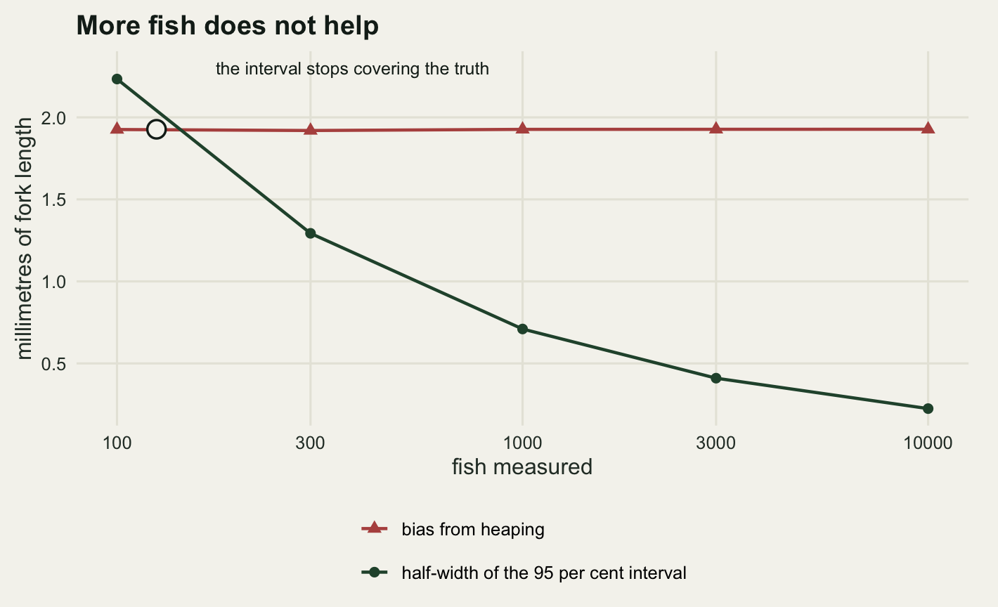 

Figure 3: The heaping bias in the mean fork length against the sample size that would be needed to see it. The bias is a fixed offset of just under two millimetres and does not move as the survey grows. The half-width of the ninety-five per cent confidence interval falls with the square root of the sample size and crosses the bias at about one hundred and twenty five fish, past which the scheme reports a wrong answer with increasing confidence.

The bias holds at -1.926 mm at a hundred fish and -1.927 mm at ten thousand, while the standard error falls from 1.14 to 0.115. The coverage of the nominal ninety-five per cent interval for the mean drops from 59.9 per cent at a hundred fish to 16.6 at three hundred, and is 0 from a thousand onwards. Past about 125 fish the interval no longer contains the truth, and every additional pass of the electrofisher makes the statement more confident and no less wrong. In the companion post the same sweep produced a mean bias indistinguishable from zero at any sample size, and the whole cost of the ruler sat in the variance where a correction could reach it.

A contrast made out of nothing

None of that would matter much for a scheme that only reports a mean with an honest interval around it. Schemes report contrasts. The restored reach against the control, this year against the baseline, the fished bank against the unfished one. A contrast is a difference of two means, and a difference of two means is safe from heaping only when both arms were heaped the same way.

The design at the top of the post guarantees they were not. The restored reach is measured first thing by a fresh crew; the control is measured at dusk. Both reaches are drawn from the same population, so the true difference is zero.

set.seed(20260808)
z_rest <- rnorm(n_reach, mu_fish, sd_fish)
z_ctrl <- rnorm(n_reach, mu_fish, sd_fish)
y_rest <- heap_record(z_rest, crew_am[1], crew_am[2], crew_am[3])
y_ctrl <- heap_record(z_ctrl, crew_pm[1], crew_pm[2], crew_pm[3])

tt_board <- t.test(round(z_rest), round(z_ctrl))
tt_sheet <- t.test(y_rest, y_ctrl)
board_diff <- unname(tt_board$estimate[1] - tt_board$estimate[2])
sheet_diff <- unname(tt_sheet$estimate[1] - tt_sheet$estimate[2])
print(round(c(board_diff = board_diff, board_p = tt_board$p.value,
              sheet_diff = sheet_diff, lower = tt_sheet$conf.int[1],
              upper = tt_sheet$conf.int[2]), 4))

board_diff    board_p sheet_diff      lower      upper 
   -0.1817     0.7724     1.4867     0.2203     2.7531 

print(signif(c(sheet_p = tt_sheet$p.value), 3))

sheet_p 
 0.0214 

print(round(c(whipple_restored = whipple(y_rest),
              whipple_control = whipple(y_ctrl)), 1))

whipple_restored  whipple_control 
           170.8            345.8 

On the board the two reaches differ by -0.182 mm with a p value of 0.772, which is the truth. On the sheet the restored reach comes out 1.49 mm longer, with a ninety-five per cent interval from 0.22 to 2.75 and a p value of 0.021. A restoration effect on juvenile trout growth, significant at the conventional level, produced by nobody doing anything wrong except getting tired.

One realisation is an anecdote, so the same experiment repeated two thousand times, alongside two controls: both reaches heaped identically, and both reaches coarsened onto different uniform grids in the manner of the companion post.

one_contrast <- function(regime) {
  za <- rnorm(n_reach, mu_fish, sd_fish)
  zb <- rnorm(n_reach, mu_fish, sd_fish)
  if (regime == "clean") {
    ya <- round(za); yb <- round(zb)
  } else if (regime == "same heaping") {
    ya <- heap_record(za, crew_pm[1], crew_pm[2], crew_pm[3])
    yb <- heap_record(zb, crew_pm[1], crew_pm[2], crew_pm[3])
  } else if (regime == "different grids") {
    ya <- round_to(za, 1); yb <- round_to(zb, 5)
  } else {
    ya <- heap_record(za, crew_am[1], crew_am[2], crew_am[3])
    yb <- heap_record(zb, crew_pm[1], crew_pm[2], crew_pm[3])
  }
  tt <- t.test(ya, yb)
  c(unname(tt$estimate[1] - tt$estimate[2]), tt$p.value)
}

set.seed(20260809)
regimes <- c("clean", "same heaping", "different grids", "different heaping")
rep_store <- lapply(regimes, function(rg) t(replicate(2000, one_contrast(rg))))
names(rep_store) <- regimes
con_res <- do.call(rbind, lapply(regimes, function(rg) {
  M <- rep_store[[rg]]
  data.frame(regime = rg, mean_contrast = mean(M[, 1]), sd_contrast = sd(M[, 1]),
             rejection = mean(M[, 2] < 0.05))
}))
print(con_res, digits = 4)

             regime mean_contrast sd_contrast rejection
1             clean      0.006411      0.6280    0.0485
2      same heaping     -0.011942      0.6589    0.0505
3   different grids     -0.010860      0.6186    0.0380
4 different heaping      1.793466      0.6564    0.7825

rej_of <- function(rg) con_res$rejection[con_res$regime == rg]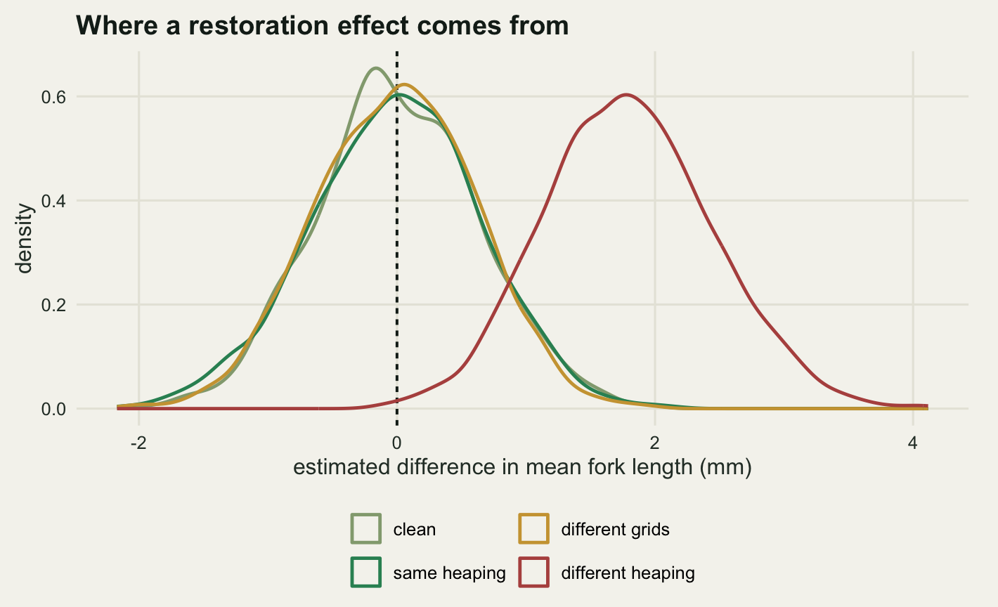

Figure 4: Sampling distribution of the estimated difference in mean fork length between two reaches drawn from the same population, over two thousand simulated survey days. Clean recording, identical heaping in both reaches and different uniform grids in the two reaches all centre on zero. Differential heaping, the restored reach measured by a fresh crew and the control at dusk, shifts the whole distribution to a difference of nearly two millimetres that is not there.

Clean recording rejects the true null 4.9 per cent of the time, identical heaping in both arms 5.1 per cent, and two different uniform grids 3.8 per cent. That third number is the companion post’s result arriving in a comparison: coarsening one arm onto a five millimetre grid and leaving the other at the millimetre changes nothing about the contrast, because neither grid moves a mean. Differential heaping rejects 78.2 per cent of the time, with an average manufactured difference of 1.793 mm.

The ecological reading is worth stating plainly. Heaping is close to harmless for a summary statistic quoted with a wide enough interval, and it is dangerous for exactly the comparisons that monitoring exists to make, because those comparisons are the places where observer, season, time of day and effort differ systematically between the things being compared. This is a different failure from the observer effects already on the site: it is not that some crews detect fewer fish or identify them differently, it is that two crews looking at the same fish on the same board write down different numbers, and the difference has a sign.

What a mixture model buys

The map from truth to record is stochastic and its parameters are unknown, so the repair has to estimate them. The idea is old: Heitjan and Rubin (1990) fit it to heaped ages, Ridout and Morgan (1991) to digit preference in biological counts, and Wang and Heitjan (2008) to self-reported cigarette counts, where the attractors are 10 and 20 and the same asymmetry question arises. Write the likelihood of a recorded value as a mixture over what the recorder might have done. A reading that is not a multiple of five can only be an honest millimetre reading, so it contributes the probability of the latent value falling in that one millimetre cell. A reading on a multiple of ten can be an honest reading, a five heap or a ten heap, and each of those is a probability of the latent value falling in a stretch of the line: for a downward ten heap, anywhere in the ten millimetres at or above the recorded value.

heap_lik <- function(y, mu, s, p10, p5, asym) {
  q5 <- (1 - p10) * p5
  q0 <- (1 - p10) * (1 - p5)
  cell <- pnorm(y + 0.5, mu, s) - pnorm(y - 0.5, mu, s)
  wd <- (1 + asym) / 2
  wu <- (1 - asym) / 2
  lik <- q0 * cell
  i5 <- (y %% 5) == 0
  i10 <- (y %% 10) == 0
  if (any(i5)) {
    v <- y[i5]
    lik[i5] <- lik[i5] + q5 * (cell[i5] +
      wd * (pnorm(v + 4.5, mu, s) - pnorm(v + 0.5, mu, s)) +
      wu * (pnorm(v - 0.5, mu, s) - pnorm(v - 4.5, mu, s)))
  }
  if (any(i10)) {
    v <- y[i10]
    lik[i10] <- lik[i10] + p10 * (cell[i10] +
      wd * (pnorm(v + 9.5, mu, s) - pnorm(v + 0.5, mu, s)) +
      wu * (pnorm(v - 0.5, mu, s) - pnorm(v - 9.5, mu, s)))
  }
  lik
}

nll_heap <- function(par, y) {
  -sum(log(pmax(heap_lik(y, par[1], exp(par[2]), plogis(par[3]),
                         plogis(par[4]), 2 * plogis(par[5]) - 1), 1e-300)))
}

fit_heap <- function(y, hess = FALSE) {
  st <- c(mean(y), log(sd(y)), 0, 0, 0)
  o <- optim(st, nll_heap, y = y, method = "Nelder-Mead",
             control = list(maxit = 3000, reltol = 1e-10))
  o <- optim(o$par, nll_heap, y = y, method = "BFGS", hessian = hess,
             control = list(maxit = 400))
  out <- c(mu = o$par[1], sigma = exp(o$par[2]), p10 = plogis(o$par[3]),
           p5 = plogis(o$par[4]), asym = 2 * plogis(o$par[5]) - 1)
  if (hess) {
    se <- suppressWarnings(tryCatch(sqrt(diag(solve(o$hessian))),
                                    error = function(e) rep(NA_real_, 5)))
    out <- c(out, se_mu = unname(se[1]))
  }
  out
}

fit_rest <- fit_heap(y_rest, hess = TRUE)
fit_ctrl <- fit_heap(y_ctrl, hess = TRUE)
print(round(rbind(restored = fit_rest, control = fit_ctrl), 4))

              mu   sigma    p10     p5 asym  se_mu
restored 78.5786 11.1183 0.1382 0.0452  0.1 0.5312
control  79.4149 10.6355 0.4638 0.2837  1.0 0.4453

con_fit <- unname(fit_rest["mu"] - fit_ctrl["mu"])
con_se <- unname(sqrt(fit_rest["se_mu"]^2 + fit_ctrl["se_mu"]^2))
print(round(c(board_ctrl = mean(round(z_ctrl)), sheet_ctrl = mean(y_ctrl),
              board_contrast = board_diff, sheet_contrast = sheet_diff,
              fitted_contrast = con_fit, fitted_se = con_se), 4))

     board_ctrl      sheet_ctrl  board_contrast  sheet_contrast fitted_contrast 
        78.8300         77.0233         -0.1817          1.4867         -0.8363 
      fitted_se 
         0.6931 

On the control reach’s six hundred fish the fit returns a mean of 79.415 mm against a board mean of 78.83, where the sheet mean was 77.023. It recovers a pull probability of 0.464 to multiples of ten against the true 0.45, having been told nothing about the recorder at all. The asymmetry comes back at 1, which is the edge of the parameter space rather than the true 0.8, and that pinning is worth watching: on this reach the fit overshoots by 0.58 mm, having started 1.81 mm out. Differencing the two reaches turns the manufactured contrast of 1.49 mm into -0.84 with a standard error of 0.69, against a board contrast of -0.18.

One survey is one draw, so the same day repeated a hundred and fifty times, fitting both reaches each time.

set.seed(20260810)
n_days <- 150
rep_res <- t(replicate(n_days, {
  za <- rnorm(n_reach, mu_fish, sd_fish)
  zb <- rnorm(n_reach, mu_fish, sd_fish)
  ya <- heap_record(za, crew_am[1], crew_am[2], crew_am[3])
  yb <- heap_record(zb, crew_pm[1], crew_pm[2], crew_pm[3])
  fa <- fit_heap(ya, hess = TRUE)
  fb <- fit_heap(yb, hess = TRUE)
  cf <- unname(fa["mu"] - fb["mu"])
  cs <- unname(sqrt(fa["se_mu"]^2 + fb["se_mu"]^2))
  tt <- t.test(ya, yb)
  c(board = mean(round(zb)), sheet = mean(yb), fitted = unname(fb["mu"]),
    se_fit = unname(fb["se_mu"]), se_sheet = sd(yb) / sqrt(n_reach),
    cover = as.numeric(abs(fb["mu"] - mu_fish) < 1.96 * fb["se_mu"]),
    con_sheet = unname(tt$estimate[1] - tt$estimate[2]),
    rej_sheet = as.numeric(tt$p.value < 0.05),
    con_fitted = cf, rej_fitted = as.numeric(abs(cf) > 1.96 * cs))
}))
n_se_ok <- sum(!is.na(rep_res[, "se_fit"]))
rep_sum <- colMeans(rep_res, na.rm = TRUE)
print(round(rep_sum, 4))

     board      sheet     fitted     se_fit   se_sheet      cover  con_sheet 
   77.9468    76.0401    77.8742     0.6927     0.4678     0.9933     1.8600 
 rej_sheet con_fitted rej_fitted 
    0.8133     0.2275     0.0616 

print(round(c(bias_sheet = unname(rep_sum["sheet"] - mu_fish),
              bias_fitted = unname(rep_sum["fitted"] - mu_fish),
              sd_fitted = sd(rep_res[, "fitted"]),
              se_inflation = unname(rep_sum["se_fit"] / rep_sum["se_sheet"]),
              usable_se = n_se_ok / n_days), 4))

  bias_sheet  bias_fitted    sd_fitted se_inflation    usable_se 
     -1.9599      -0.1258       0.5722       1.4808       0.9933 

Across 150 survey days the control reach’s sheet mean sits -1.96 mm below the truth and the fitted mean -0.126 mm, with the interval covering the truth 99.3 per cent of the time. That coverage is over rather than under nominal: the fitted means scatter with a standard deviation of 0.572 mm while the fit reports 0.693, so the intervals are wider than they need to be. The manufactured contrast falls from 1.86 mm to 0.227, and the false positive rate from 81.3 per cent to 6.2 per cent. That is most of the damage undone, and it is still not a nominal test.

The price is precision. The standard error of the fitted mean is 1.481 times the naive one, because the likelihood has to work out what the recorder was doing before it can say anything about the fish, and on 0.7 per cent of the days it returns no standard error at all: the asymmetry pins at its bound, the observed information is singular in that direction, and inverting the Hessian gives nothing.

The companion post’s interval-censored fit paid none of that, and the reason is structural. There the grid was known, the map from truth to record was deterministic, and the likelihood had two parameters, both of them about the biology. Here three of the five parameters describe the observer, and the asymmetry in particular is identified only through the shape of the assumed latent distribution, because the digit table is blind to it.

Where the repair stops working

The model above assumes that whether a reading gets heaped is unrelated to how long the fish actually was. Drop that and the whole thing collapses, and the field version of dropping it is ordinary. The crew works upstream through the day, the larger fish are in the upper pools, and the measuring gets sloppier as the light goes. Heaping probability is then a function of the very quantity being estimated.

make_day <- function(n) {
  z <- rnorm(n, mu_fish, sd_fish)
  late <- runif(n) < plogis(1.4 * (z - mu_fish) / sd_fish)
  y <- numeric(n)
  y[late] <- heap_record(z[late], crew_pm[1], crew_pm[2], crew_pm[3])
  y[!late] <- heap_record(z[!late], crew_am[1], crew_am[2], crew_am[3])
  list(z = z, y = y, late = late)
}

set.seed(20260811)
day <- make_day(4000)
fit_pool <- fit_heap(day$y)
fit_early <- fit_heap(day$y[!day$late])
fit_late <- fit_heap(day$y[day$late])
w_late <- mean(day$late)
mu_aware <- (1 - w_late) * fit_early["mu"] + w_late * fit_late["mu"]
print(round(c(board = mean(round(day$z)), sheet = mean(day$y),
              pooled_fit = unname(fit_pool["mu"]),
              session_aware = unname(mu_aware), share_late = w_late), 4))

        board         sheet    pooled_fit session_aware    share_late 
      78.1823       77.1120       76.0226       78.1690        0.5082 

print(round(c(pooled_asym = unname(fit_pool["asym"]),
              early_asym = unname(fit_early["asym"]),
              late_asym = unname(fit_late["asym"])), 4))

pooled_asym  early_asym   late_asym 
    -0.7312      0.3299      0.7879 

The board mean is 78.182 mm. The sheet mean is 77.112, low by 1.07. The pooled mixture fit returns 76.023, which is 2.16 mm low: worse than not correcting at all. Its estimated asymmetry is -0.731, against a truth that is downward in both sessions, 0.2 and 0.8. A confidently wrong sign on that parameter is the one visible symptom, and it is a weak one, since the same parameter also pins at its upper bound on well behaved data.

The reason is a single broken assumption. In the ignorable case the readings that kept their fine digits are a random sample of the population, so they anchor the latent mean. Here they are not.

set.seed(20260812)
z_ig <- rnorm(40000, mu_fish, sd_fish)
y_ig <- heap_record(z_ig, crew_pm[1], crew_pm[2], crew_pm[3])
big_day <- make_day(40000)
anchor <- c(
  ignorable = mean(round(z_ig)[(y_ig %% 5) != 0]) - mean(round(z_ig)),
  non_ignorable = mean(round(big_day$z)[(big_day$y %% 5) != 0]) -
    mean(round(big_day$z)))
print(round(anchor, 4))

    ignorable non_ignorable 
       0.0964       -2.1457 

Under ignorable heaping the fish that kept a fine digit average 0.096 mm from the population mean. Under the upstream story they average -2.146 mm from it, because the fish measured carefully are the small ones. The likelihood believes the anchor, puts the latent mean down there, and then has to explain a mass of readings on multiples of ten that sit above it, which it does by concluding that the recorders rounded upwards. Every part of that is internally consistent and every part of it is wrong.

There is a way out and it is not statistical. Split the day into its two sessions and the mechanism becomes ignorable within each one, because inside a session the pull probability no longer depends on the length.

print(round(c(board = mean(round(day$z)),
              early_fit = unname(fit_early["mu"]),
              early_board = mean(round(day$z[!day$late])),
              late_fit = unname(fit_late["mu"]),
              late_board = mean(round(day$z[day$late])),
              combined = unname(mu_aware)), 3))

      board   early_fit early_board    late_fit  late_board    combined 
     78.182      72.407      72.411      83.744      83.766      78.169 

The two sessions have genuinely different mean lengths, 72.41 and 83.77 mm, because the assignment to session depends on size. Fitting each separately and recombining by the session sizes gives 78.169 mm against a board mean of 78.182. The correction works, and the only thing it needed was a column on the recording sheet saying which session each fish came from.

What the numbers cannot tell you

The recorded lengths carry the fact of heaping and nothing else. They do not say who wrote them, when, with which board, or whether the recorder’s habit changed as the light went, and the repair above needs exactly that. A pooled fit to a mixed day is not merely less accurate than a session-aware one; on the simulation above it moved the estimate 1.09 mm further from the truth than doing nothing. There is no diagnostic in the numbers that distinguishes the two situations with any confidence, because both produce the same tall bars on 0 and 5.

Three cheap habits close most of the gap and none of them is a statistical method. Record the observer, as an identifier on every row rather than a note at the top of the sheet, so heaping can be estimated within observer and so observer can be crossed with treatment instead of confounded with it. Record the instrument, because a board with labelled centimetres and a board with labelled millimetres produce different attractor sets from the same fish. And keep one digit more than anybody thinks is useful: the resolution that looks like false precision in the field is the resolution that leaves the terminal digit free to carry information, and a scheme that records to the nearest five millimetres because that is all the biology needs has thrown away the only witness it had.

Heitjan and Rubin (1991) give the general condition, and the useful version of it here is that the heaping may depend on anything recorded and must not depend on the unrecorded true value.

Two limits on what was measured here. The mechanism is a caricature: real recorders have richer attractor sets, they heap differently in different parts of the range, and the asymmetry itself drifts through the day. And the mixture fit was given the correct family for the latent distribution. A length-frequency sample from a real river is a mixture of age classes rather than a single normal, so the shape that identifies the asymmetry is itself being estimated, and the standard errors quoted above are optimistic in the direction that matters.

What to take away

Heaping is detectable from the numbers alone, and cheaply. The Whipple index has a known null distribution, standard deviation two hundred over the square root of the sample size, so a reach of 600 fish flags anything above 113.3. That test caught 59 per cent of cases where only four per cent of readings were pulled to a round number, against 49 per cent for the omnibus chi-square on the ten digits.

Detection is not diagnosis. Two recording habits with identical digit tables, tested at two hundred thousand fish with a p value of 0.758, had means 1.922 mm apart, one of them unbiased. The bias runs at 0.241 mm per tenth of downward preference, and unlike the uniform grid of the companion post it is an offset rather than extra spread: -1.926 mm at a hundred fish and -1.927 at ten thousand, with interval coverage falling to zero past about 125 fish.

The damage lands on contrasts. Two reaches from one population, measured by a fresh crew and a tired one, produced a difference of 1.49 mm with a p value of 0.021 in the single survey and a false positive rate of 78.2 per cent over two thousand of them, against 3.8 per cent when the two arms differed by a uniform grid instead.

The mixture repair works when the mechanism is ignorable, returning a bias of -0.126 mm against the sheet’s -1.96, and pulling the false positive rate on the contrast from 81.3 per cent down to 6.2, at the cost of a standard error 1.48 times as wide. When heaping depends on the true length it does not merely fail, it overshoots: 76.02 mm against a board mean of 78.18, further out than the uncorrected 77.11. Splitting the same data by measuring session recovered 78.17. The repair that worked was a column on the recording sheet, not a model.

References

Ridout MS, Morgan BJT 1991 Biometrics 47(4):1423-1433 (10.2307/2532396)

Heitjan DF, Rubin DB 1990 Journal of the American Statistical Association 85(410):304-314 (10.1080/01621459.1990.10476202)

Heitjan DF, Rubin DB 1991 The Annals of Statistics 19(4):2244-2253 (10.1214/aos/1176348396)

Wang H, Heitjan DF 2008 Statistics in Medicine 27(19):3789-3804 (10.1002/sim.3281)

Camarda CG, Eilers PHC, Gampe J 2008 Statistical Modelling 8(4):385-401 (10.1177/1471082X0800800404)

Roberts JM, Brewer DD 2001 Journal of Applied Statistics 28(7):887-896 (10.1080/02664760120074960)

A’Hearn B, Baten J, Crayen D 2009 The Journal of Economic History 69(3):783-808 (10.1017/S0022050709001120)

Marques TA 2004 Biometrics 60(3):757-763 (10.1111/j.0006-341X.2004.00226.x)

Related tutorials

• Rounded and coarsened measurements
• Fitting a mixture of normals in R
• Checking a distance sampling model
• Measurement error and regression dilution