Checking published summary statistics

A rounded mean or t value from a paper is a band, not a point. GRIM, SD bounds and recomputed p values in R, with the false alarms a missing sample creates.

A synthesis of clutch size in cavity nesting tits is at the extraction stage. The spreadsheet has one row per population, and each row holds what the paper printed: a mean clutch size, a standard deviation, the number of nests, and for the papers that compared nest boxes with natural cavities, a t statistic, its degrees of freedom and a p value. One row reads: 24 nests, mean clutch 3.47 eggs. Nobody can lay a fraction of an egg, so the 24 clutches sum to a whole number, and 83 eggs over 24 nests is 3.46 while 84 eggs is 3.50. No whole number of eggs divided by 24 rounds to 3.47.

That arithmetic is the GRIM test of Brown and Heathers (2017), and it is the simplest of a family of checks that ask whether the numbers a paper printed can have come from any data set at all. They do not need the raw data. They use only the fact that the printed numbers are rounded functions of something with structure: counts are integers, scores sit on a bounded scale, and a p value is a fixed function of a t statistic and its degrees of freedom. The catch, and the subject of this post, is that rounding throws information away, so a printed number corresponds to a band of possible true values rather than a single one. Each check below is only as sharp as that band is narrow, and the band is often wide.

The grain of a measurement has come up twice on this site already, but in the other direction. Rounded and coarsened measurements treats the rounding of your own field data, the variance it adds and the likelihood that repairs it; digit preference and heaping treats recorders who drift towards round numbers. In both, the data are in hand and the question is what the grain did to them. Here the data are in someone else’s filing cabinet and the question is whether the printed summaries are internally consistent. The closest neighbour is effect sizes from incomplete reports, which recovers a standard deviation from a median and quartiles at the same extraction stage; this post is the check that should come before any such recovery.

One point of tone before any code. An inconsistency is a flag that something in the printed numbers does not fit together. The usual cause is mundane: a typographical error, a table updated after one row was dropped, a sample size taken from the methods rather than from the analysis. The final third of the post measures how often an entirely honest mean fails GRIM for exactly that last reason, and the answer is often enough that a flag on its own should lead to a polite question to the authors and nothing else.

library(ggplot2)
library(patchwork)

te_paper  <- "#f5f4ee"
te_ink    <- "#16241d"
te_body   <- "#2c3a31"
te_forest <- "#275139"
te_rust   <- "#b5534e"
te_gold   <- "#c9b458"
te_line   <- "#dad9ca"

theme_datasheet <- function() {
  theme_minimal(base_size = 12) +
    theme(plot.background  = element_rect(fill = te_paper, colour = NA),
          panel.background = element_rect(fill = te_paper, colour = NA),
          panel.grid.major = element_line(colour = te_line, linewidth = 0.3),
          panel.grid.minor = element_blank(),
          text             = element_text(colour = te_body),
          plot.title       = element_text(colour = te_ink, face = "bold"),
          plot.subtitle    = element_text(colour = te_body),
          axis.text        = element_text(colour = te_body))
}

A mean of integers lives on a grid

If n integers sum to S, their mean is S over n, and the printed mean is that fraction rounded to d decimals. A printed mean m is consistent with n when some whole number S gives a fraction inside the rounding interval of m, which under the usual round half up rule is from m minus half a unit in the last decimal up to, but not including, m plus half a unit. The function below does this in integer arithmetic, so no floating point representation of a value such as 3.475 can decide the answer. It finds the smallest S that reaches the bottom of the interval and asks whether that S is still below the top. A lenient flag closes the top of the interval, which accepts a mean that sits exactly on a rounding tie whichever way the author’s software broke it.

grim_ok <- function(m_rep, n, d, lenient = FALSE) {
  sc   <- 10^d
  m_int <- round(m_rep * sc)                      # printed mean in units of the last decimal
  s_lo <- -((-(2 * m_int - 1) * n) %/% (2 * sc))  # smallest S with S / n >= m - half a unit
  if (lenient) 2 * s_lo * sc <= (2 * m_int + 1) * n else 2 * s_lo * sc < (2 * m_int + 1) * n
}

# brute force: every sum from 0 to 20 n, rounded half up, compared with the function
grim_brute <- function(m_rep, n, d) {
  s_all <- 0:(20 * n)
  any(floor(s_all * 10^d / n + 0.5) == round(m_rep * 10^d))
}
set.seed(2017)
n_check <- 3000
check_n <- sample(2:150, n_check, replace = TRUE)
check_m <- round(runif(n_check, 0, 15), 2)
agree_all <- all(mapply(grim_brute, check_m, check_n, 2) == grim_ok(check_m, check_n, 2))

clutch_n <- 24; clutch_m <- 3.47
clutch_lo <- floor(clutch_m * clutch_n); clutch_hi <- clutch_lo + 1
clutch_ok <- grim_ok(clutch_m, clutch_n, 2)

Against an exhaustive search over every sum from zero to twenty times n, the function agrees on all 3000 random pairs of printed mean and sample size: no disagreements. For the clutch row the two nearest sums are 83 and 84 eggs, giving 3.4583 and 3.5000, and the function returns inconsistent.

The whole structure is easier to see as a map. For each sample size along the bottom and each possible pair of printed decimals up the side, a cell is consistent if some sum reaches it.

map_n   <- 1:120
map_dec <- 0:99
grim_map <- expand.grid(n = map_n, dec = map_dec)
grim_map$ok <- grim_ok(3 + grim_map$dec / 100, grim_map$n, 2)
grim_map$status <- ifelse(grim_map$ok, "consistent", "inconsistent")

ggplot(grim_map, aes(n, dec / 100, fill = status)) +
  geom_tile() +
  geom_vline(xintercept = 100, colour = te_ink, linewidth = 0.5, linetype = "dashed") +
  scale_fill_manual(values = c(consistent = te_forest, inconsistent = te_paper)) +
  scale_x_continuous(breaks = seq(0, 120, 20), expand = c(0, 0)) +
  scale_y_continuous(breaks = seq(0, 1, 0.2), expand = c(0, 0)) +
  labs(x = "sample size n", y = "decimal part of the printed mean", fill = NULL,
       title = "The grid of reachable means",
       subtitle = "two decimals, round half up; dark cells can come from integer data") +
  theme_datasheet() +
  theme(legend.position = "top",
        legend.key = element_rect(colour = te_ink, linewidth = 0.3))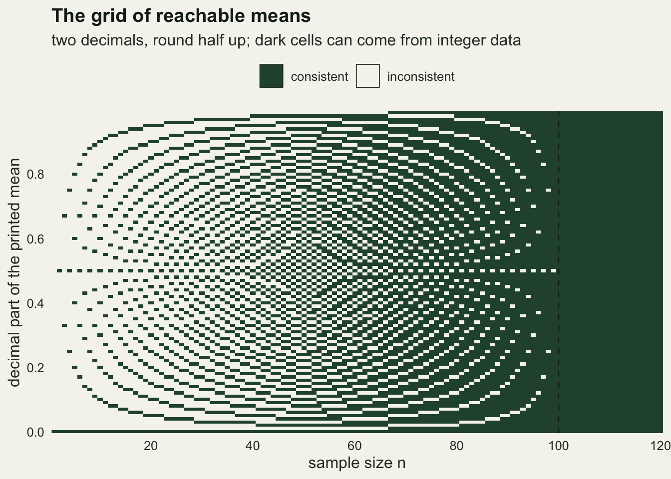

Figure 1: Which two-decimal means are reachable from integer data, by sample size. Every column at or beyond one hundred is fully consistent.

How often the grid can catch anything

The map has a closed form. In any unit interval there are 10 to the power d possible printed decimals and n fractions S over n. If n is smaller than 10 to the d, consecutive fractions are further apart than one rounding interval, so they land on n different printed values and the remaining ones are unreachable. If n is at least 10 to the d, every rounding interval contains a fraction and nothing is unreachable. So the share of printed decimals that GRIM can reject is one minus n over 10 to the d, floored at zero. It is the probability that a mean with random final digits is flagged, which is the most GRIM can offer: a detection rate for a mean that is wrong in its last digits.

grim_power <- function(n, d) pmax(0, 1 - n / 10^d)

dec_grid <- function(d) 3 + (0:(10^d - 1)) / 10^d
exact_gap <- sapply(1:3, function(d) {
  n_set <- 1:(10^d + 5)
  share <- sapply(n_set, function(n) mean(!grim_ok(dec_grid(d), n, d)))
  max(abs(share - grim_power(n_set, d)))
})

n_sim <- 10000
set.seed(363)
sim24_m   <- round(runif(n_sim, 1, 9), 2)
flag24    <- mean(!grim_ok(sim24_m, clutch_n, 2))
flag24_se <- sqrt(flag24 * (1 - flag24) / n_sim)

pair_n  <- sample(5:150, n_sim, replace = TRUE)
pair_m  <- round(runif(n_sim, 1, 9), 2)
pair_flag <- mean(!grim_ok(pair_m, pair_n, 2))
pair_cf   <- mean(grim_power(pair_n, 2))
pair_z    <- (pair_flag - pair_cf) / sqrt(pair_cf * (1 - pair_cf) / n_sim)
share_big <- mean(pair_n >= 100)

Counted exhaustively over every printed decimal, the closed form and the direct count differ by nothing, in every case, for one, two and three decimals and every n up to just past 10 to the d. For the clutch row it gives 0.76. Ten thousand means with random two-decimal endings, checked against n of 24, were flagged at a rate of 0.7598, with a Monte Carlo standard error of 0.0043. A second set of ten thousand pairs, with n drawn uniformly from 5 to 150, was flagged at 0.3158 against a closed form average of 0.3147, a difference of 0.2 standard errors. In that set 0.35 of the pairs had n of 100 or more and contributed no flags at all.

The consequence is blunt. At two decimals the test goes blind at a sample of 100 and is weak well before that: n of 50 leaves 0.50 of all printed endings reachable. At one decimal it is blind from n of 10. A third printed decimal would stretch the range to 1000, but means are rarely printed that way. The test also needs integer data with a known number of items per observation. Clutch sizes, counts of individuals and ordinal scores qualify. A mean body mass read from a balance to 0.01 g and printed to two decimals does not, and neither does a cover percentage averaged from fractional estimates, because the recorded values are finer than the printed mean. Cover recorded to the nearest whole per cent does qualify, as long as the mean was computed from those recorded values.

Ties, and the sample sizes that hide them

The closed form assumes one rounding rule. The rules differ only when S over n sits exactly halfway between two printed values, as 3 over 8, which is 0.375, sits between 0.37 and 0.38. Round half up prints 0.38; round half to even prints 0.38 as well, but 0.125 goes to 0.12 under half to even and 0.13 under half up; and a spreadsheet may do something else again once floating point is involved. A checker does not know which rule the author used, so the fair version accepts both neighbours of a tie. That is the lenient flag.

gcd_int <- function(a, b) ifelse(b == 0, a, gcd_int(b, a %% b))
two_adic <- function(n) { v <- 0; while (n %% 2 == 0) { n <- n / 2; v <- v + 1 }; v }

# ties exist exactly when n has more factors of two than 10^d; there are gcd(n, 10^d) of them
tie_count <- function(n, d) if (two_adic(n) > d) gcd_int(n, 10^d) else 0
grim_power_lenient <- function(n, d) pmax(0, 1 - (n + tie_count(n, d)) / 10^d)

n_tie_set <- 1:200
len_count <- sapply(n_tie_set, function(n) mean(!grim_ok(dec_grid(2), n, 2, lenient = TRUE)))
len_form  <- sapply(n_tie_set, grim_power_lenient, d = 2)
tie_gap   <- max(abs(len_count - len_form))
tie_ns    <- n_tie_set[n_tie_set < 100 & sapply(n_tie_set, tie_count, d = 2) > 0]

flag24_len <- mean(!grim_ok(sim24_m, clutch_n, 2, lenient = TRUE))
len_40 <- grim_power_lenient(40, 2); len_80 <- grim_power_lenient(80, 2)

power_tab <- data.frame(n = rep(1:120, 2),
                        power = c(grim_power(1:120, 2), sapply(1:120, grim_power_lenient, d = 2)),
                        rule = rep(c("one fixed rounding rule", "either neighbour of a tie"), each = 120))
power_tab$rule <- factor(power_tab$rule, levels = c("one fixed rounding rule", "either neighbour of a tie"))

Ties arise only when S over n has one more decimal than is printed and that decimal is a five. Writing n over the greatest common divisor of n and 10 to the d, a tie needs that reduced denominator to be even, which happens exactly when n contains more factors of two than 10 to the d does, and there are then as many ties per unit interval as that greatest common divisor. At two decimals the sample sizes below 100 with ties are the multiples of eight, 12 of them. This lenient closed form matches an exhaustive count for every n from 1 to 200 exactly.

The clutch row is one of the affected cases. Twenty-four is a multiple of eight, so the fair detection rate at n of 24 is 0.72, not 0.76, and the same ten thousand random means were flagged at 0.7196 under the lenient rule. The effect is largest at multiples of 40, where there are 20 ties per unit interval instead of 4: at n of 40 the lenient rate is 0.40 against 0.60, and at n of 80 it is 0.00, so a sample of 80 cannot fail a lenient GRIM check at two decimals at all. The 3.47 from 24 nests is not near a tie and fails under either rule.

ggplot(power_tab, aes(n, power, colour = rule)) +
  geom_line(data = subset(power_tab, rule == "one fixed rounding rule"), linewidth = 0.9) +
  geom_point(data = subset(power_tab, rule == "either neighbour of a tie" & n %% 8 == 0 & n < 100),
             size = 2.4) +
  annotate("point", x = clutch_n, y = flag24, shape = 4, size = 3.5, stroke = 1.1, colour = te_ink) +
  annotate("text", x = clutch_n + 4, y = flag24 + 0.07, hjust = 0,
           label = "simulated, n = 24", colour = te_ink, size = 3.6) +
  scale_colour_manual(values = c("one fixed rounding rule" = te_forest,
                                 "either neighbour of a tie" = te_rust)) +
  scale_x_continuous(breaks = seq(0, 120, 20)) +
  coord_cartesian(ylim = c(0, 1)) +
  labs(x = "sample size n", y = "share of printed means GRIM can reject", colour = NULL,
       title = "Blind from one hundred, and earlier at multiples of eight",
       subtitle = "red points: sample sizes with rounding ties, checked leniently") +
  theme_datasheet() +
  theme(legend.position = "top")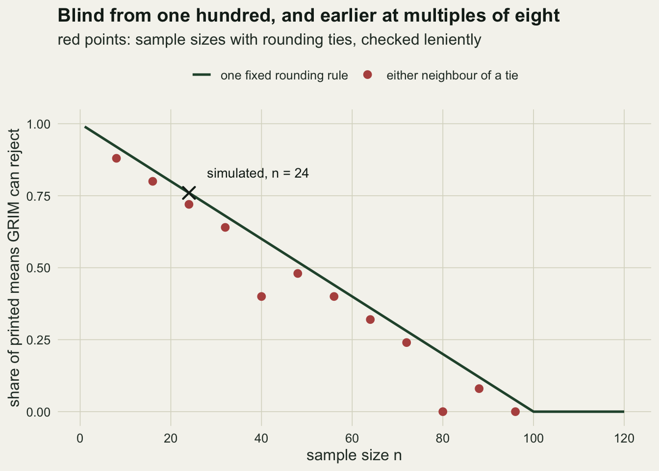

Figure 2: Share of two-decimal printed means that GRIM can reject, under one fixed rounding rule and under the fair rule that accepts both neighbours of a tie.

A missing nest looks like an error

The sample size in the check is the one the paper printed, and the printed n is not always the n behind the mean. A table heading says 24 nests because 24 were monitored; one clutch was predated before completion and left out of the mean. The mean is then a whole number of eggs divided by 23, and it is checked against 24.

The simulation below generates honest clutch data, two eggs plus a Poisson count with mean 1.5, drops k nests at random, prints the mean of the rest correctly to two decimals, and checks it against the full n with the lenient rule. These are design constants fixed before the first run. A second computation asks what a cautious checker loses by accepting any n from the printed one down to the printed one minus j.

honest_flag <- function(n_rep, k_miss, n_rep_sim = 10000) {
  n_use <- n_rep - k_miss
  sums  <- rowSums(matrix(2 + rpois(n_rep_sim * n_use, 1.5), n_rep_sim))
  m_rep <- floor(sums * 100 / n_use + 0.5) / 100
  mean(!grim_ok(m_rep, n_rep, 2, lenient = TRUE))
}
k_set <- 0:3
set.seed(1205)
fa_24 <- sapply(k_set, function(k) honest_flag(24, k))
fa_60 <- sapply(k_set, function(k) honest_flag(60, k))
fa_se_max <- sqrt(0.25 / n_sim)

allow_power <- function(n, j_max, d = 2) {
  reach <- rep(FALSE, 10^d)
  for (j in 0:j_max) reach <- reach | grim_ok(dec_grid(d), n - j, d, lenient = TRUE)
  mean(!reach)
}
n_allow <- c(12, 24, 36, 48, 60)
allow_tab <- expand.grid(n = n_allow, j_max = 0:3)
allow_tab$power <- mapply(allow_power, allow_tab$n, allow_tab$j_max)
pw <- function(n, j) allow_tab$power[allow_tab$n == n & allow_tab$j_max == j]

fa_tab <- data.frame(k = rep(k_set, 2), rate = c(fa_24, fa_60),
                     n_print = factor(rep(c("printed n = 24", "printed n = 60"), each = length(k_set))))

With the right n, no honest mean was flagged: 0.0000 at 24 and 0.0000 at 60, which is only the implementation confirming itself. With one nest silently missing, 0.8202 of honest means from a printed 24 were flagged, and 0.6009 from a printed 60. Two missing gave 0.9101 and 0.3660, three missing 0.6241 and 0.4109. The rates do not rise steadily with k, because they depend on how the grids for n and n minus k happen to overlap, which is arithmetic rather than a trend. The Monte Carlo standard error of every rate is at most 0.0050.

A single unreported exclusion produces false alarms at a rate as large as the detection rate or larger: 0.82 against a detection rate of 0.72 at a printed 24, and 0.60 against 0.40 at 60. The detection rate is computed for endings drawn evenly over the grid, and honest means from 23 nests are not such a draw, which is why the two rates need not match. The cautious repair, accepting any n down to two below the printed one, removes the false alarms for up to two exclusions and pays in power: at a printed n of 24 the share of random endings that can still be rejected falls from 0.72 to 0.38, and at 60 from 0.40 to 0.08.

p_fa <- ggplot(fa_tab, aes(k, rate, colour = n_print)) +
  geom_line(linewidth = 0.9) +
  geom_point(size = 2.6) +
  scale_colour_manual(values = c("printed n = 24" = te_rust, "printed n = 60" = te_gold)) +
  scale_x_continuous(breaks = k_set) +
  coord_cartesian(ylim = c(0, 1)) +
  labs(x = "nests missing from the mean", y = "honest means flagged", colour = NULL,
       title = "False alarms") +
  theme_datasheet() +
  theme(legend.position = "top")

p_allow <- ggplot(allow_tab, aes(j_max, power, group = factor(n))) +
  geom_line(colour = te_forest, linewidth = 0.8) +
  geom_point(colour = te_forest, size = 2.2) +
  geom_text(data = subset(allow_tab, j_max == 0), aes(label = paste("n =", n)),
            hjust = 1.2, size = 3.3, colour = te_ink) +
  scale_x_continuous(breaks = 0:3, limits = c(-0.7, 3.1)) +
  coord_cartesian(ylim = c(0, 1)) +
  labs(x = "exclusions allowed for, j", y = "share of endings still rejectable",
       title = "Cost of the allowance") +
  theme_datasheet()

p_fa + p_allow + plot_annotation(theme = theme_datasheet())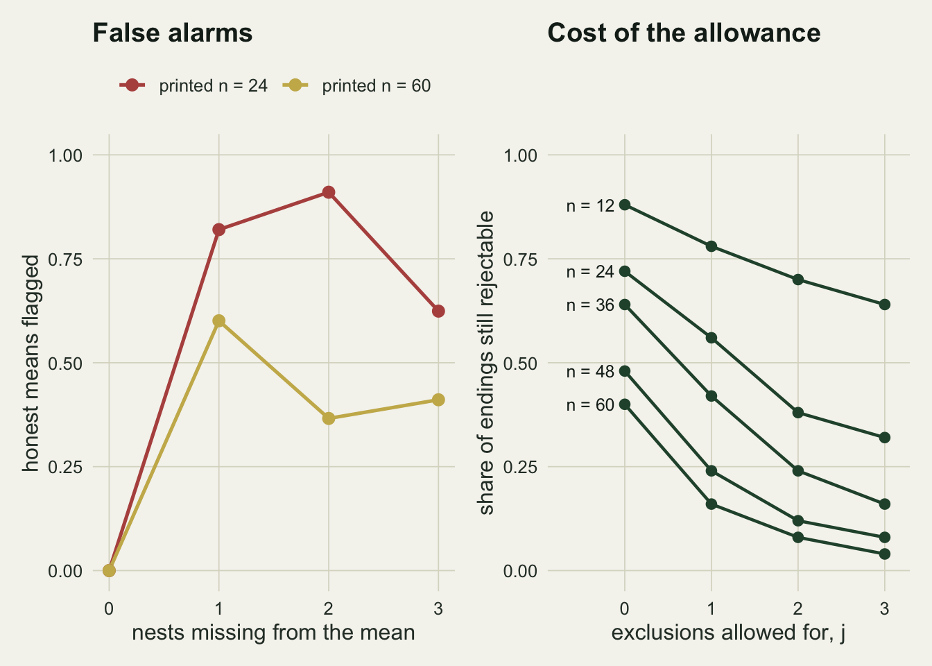

Figure 3: Left: share of honest clutch means that fail GRIM when k nests are left out of the mean but not out of the printed n. Right: what allowing for up to j excluded nests leaves of the test.

A mean and a standard deviation on a bounded scale

Sample size and mean are not the only numbers that must fit together. Given n integer scores between a lower and an upper bound that sum to S, the standard deviation cannot be arbitrarily small or large. The smallest spread puts every score at the floor or ceiling of the mean, because moving two scores that differ by two or more one step towards each other always reduces the sum of squares. The largest puts as many scores as possible at the upper bound, the rest at the lower bound, and at most one score in between, by the same exchange argument run in reverse.

The bounds are not the whole story, because the standard deviation is granular too. The sum of squares of integers is an integer, so for a fixed S the variance can take only a finite set of values, and not every integer between the two extreme sums of squares is reachable. The exact set comes from a short dynamic programme over the observations: after each score is added, a logical matrix records which pairs of sum and sum of squares are possible. This is the cheap, exact end of what SPRITE (Heathers and colleagues 2018) does by search; SPRITE reconstructs whole candidate samples, while the programme below only says whether a printed pair of mean and standard deviation is possible at all. The same question for a mean and a standard deviation has been published as the GRIMMER test (Anaya 2016); the programme here is a brute-force version of it for a small bounded scale.

The example is a crown defoliation score from 0 to 4, recorded on 20 beech trees, printed as a mean of 3.60 with a standard deviation of 1.10, 1.20 or 1.30. The closed form bounds and the dynamic programme are both checked against complete enumeration of every sample of up to six trees before they are used.

sd_bounds <- function(s_sum, n, lo, hi) {
  q <- s_sum %/% n; r <- s_sum - q * n
  ss_min <- (n - r) * q^2 + r * (q + 1)^2
  k_hi <- (s_sum - n * lo) %/% (hi - lo)
  if (k_hi >= n) {
    ss_max <- n * hi^2
  } else {
    mid <- s_sum - k_hi * hi - (n - k_hi - 1) * lo
    ss_max <- k_hi * hi^2 + (n - k_hi - 1) * lo^2 + mid^2
  }
  sqrt(c(min = (ss_min - s_sum^2 / n) / (n - 1), max = (ss_max - s_sum^2 / n) / (n - 1)))
}

# reach[S + 1, SS + 1] is TRUE if some n scores in lo:hi have sum S and sum of squares SS
reach_ss <- function(n, lo, hi) {
  s_top <- n * hi; ss_top <- n * hi^2
  cur <- matrix(FALSE, s_top + 1, ss_top + 1); cur[1, 1] <- TRUE
  for (i in seq_len(n)) {
    nxt <- matrix(FALSE, s_top + 1, ss_top + 1)
    idx <- which(cur, arr.ind = TRUE)
    for (v in lo:hi) {
      moved <- cbind(idx[, 1] + v, idx[, 2] + v^2)
      nxt[moved] <- TRUE
    }
    cur <- nxt
  }
  cur
}

enum_gap <- 0; dp_match <- TRUE
for (n in 2:6) {
  all_samples <- as.matrix(expand.grid(rep(list(0:4), n)))
  s_row <- rowSums(all_samples); sd_row <- apply(all_samples, 1, sd)
  for (s_val in unique(s_row)) {
    obs <- range(sd_row[s_row == s_val])
    enum_gap <- max(enum_gap, abs(sd_bounds(s_val, n, 0, 4) - obs))
  }
  enum_mat <- matrix(FALSE, 4 * n + 1, 16 * n + 1)
  enum_mat[cbind(s_row + 1, rowSums(all_samples^2) + 1)] <- TRUE
  dp_match <- dp_match && identical(enum_mat, reach_ss(n, 0, 4))
}

tree_n <- 20; tree_m <- 3.60
tree_reach <- reach_ss(tree_n, 0, 4)
tree_s <- which(floor((0:(4 * tree_n)) * 100 / tree_n + 0.5) == round(tree_m * 100)) - 1
tree_b <- sd_bounds(tree_s, tree_n, 0, 4)
sd_of <- function(s_val, ss) sqrt((ss - s_val^2 / tree_n) / (tree_n - 1))
tree_sds <- sort(sd_of(tree_s, which(tree_reach[tree_s + 1, ]) - 1), decreasing = TRUE)

sd_printed <- c(1.10, 1.20, 1.30)
sd_ok <- sapply(sd_printed, function(x) any(tree_sds >= x - 0.005 & tree_sds < x + 0.005))
k_top <- (tree_s - 0) %/% 4

# the same top gap at a central mean: step in sum of squares and step in SD
top_two <- function(s_val) {
  ss <- sort(which(tree_reach[s_val + 1, ]) - 1, decreasing = TRUE)[1:2]
  c(ss_step = ss[1] - ss[2], sd_gap = sd_of(s_val, ss[1]) - sd_of(s_val, ss[2]))
}
mid_s   <- 2 * tree_n
gap_mid <- top_two(mid_s)
gap_hi  <- top_two(tree_s)

band_tab <- do.call(rbind, lapply(0:(4 * tree_n), function(s_val) {
  b <- sd_bounds(s_val, tree_n, 0, 4)
  data.frame(mean = s_val / tree_n, sd_min = b[["min"]], sd_max = b[["max"]])
}))
dot_tab <- do.call(rbind, lapply(0:(4 * tree_n), function(s_val) {
  ss <- which(tree_reach[s_val + 1, ]) - 1
  data.frame(mean = s_val / tree_n, sd = sd_of(s_val, ss))
}))
sd_pts <- data.frame(mean = tree_m, sd = sd_printed,
                     status = ifelse(sd_ok, "printed SD possible", "printed SD impossible"))

Across every sample of two to six scores the closed form bounds match the enumerated minimum and maximum to within 1.2e-15, and the dynamic programme reproduces the enumerated set of sum and sum of squares pairs exactly. For 20 trees a printed 3.60 allows only a sum of 72, and that sum allows a standard deviation from 0.503 to 1.231. Inside those bounds the reachable values are discrete, and the gap at the top is wide: the largest is 1.2312, with 18 trees at 4 and the rest at 0, and the next is 1.0954.

The three printed values fare differently, for three different reasons. A printed 1.10 is possible, because 1.0954 rounds to it. A printed 1.20 lies inside the bounds and is still impossible, since no reachable value falls between 1.195 and 1.205. A printed 1.30 is above the largest possible value and impossible. A check that used only the bounds would pass the middle one. The high mean is what widens the gap, though not through a larger step in the sum of squares. Moving one tree off 4 and one off 0 changes the sum of squares by 6 at a mean of 3.60 and by 6 at a mean of 2.00. Close to a scale bound the largest standard deviation is small, and the same step in the sum of squares is a larger step in the standard deviation: the top gap is 0.1357 at 3.60 against 0.0784 at 2.00.

ggplot(band_tab, aes(mean)) +
  geom_ribbon(aes(ymin = sd_min, ymax = sd_max), fill = te_forest, alpha = 0.15) +
  geom_line(aes(y = sd_max), colour = te_forest, linewidth = 0.8) +
  geom_line(aes(y = sd_min), colour = te_forest, linewidth = 0.8) +
  geom_point(data = dot_tab, aes(y = sd), colour = te_forest, size = 0.35, alpha = 0.6) +
  geom_point(data = sd_pts, aes(y = sd, colour = status), size = 3.2, shape = 18) +
  scale_colour_manual(values = c("printed SD possible" = te_gold, "printed SD impossible" = te_rust)) +
  labs(x = "mean score of 20 trees", y = "standard deviation", colour = NULL,
       title = "Spread is bounded by the scale, and granular inside it",
       subtitle = "lines: closed form bounds; dots: every reachable standard deviation") +
  theme_datasheet() +
  theme(legend.position = "top")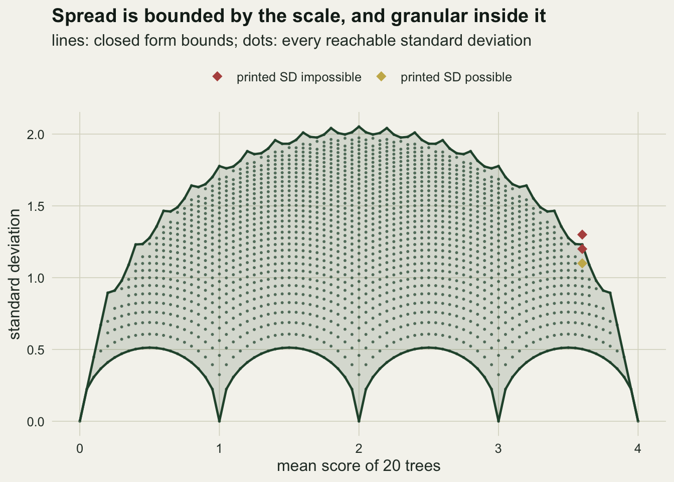

Figure 4: Standard deviations reachable by 20 integer scores between 0 and 4, for every possible mean: the closed form bounds and the discrete values between them. Three printed standard deviations for a mean of 3.60 are marked.

A rounded t gives a band of p values

The nest box comparison in the same paper prints t = 2.05 with 38 degrees of freedom and p = 0.047. A two-sided p value is twice the upper tail of the t distribution beyond the absolute value of t, and that is strictly decreasing in the absolute value, so the rounding interval of t maps to an interval of p by evaluating the two ends and swapping them. This is the logic of statcheck (Nuijten and colleagues 2016), which counts a reported p as consistent when it can be recomputed from some test statistic that rounds to the printed one. The only edge case is a printed t of zero, whose interval crosses zero; the lower end of the absolute value is then zero and the upper end of p is one.

p_band <- function(t_rep, df, dec) {
  half <- 0.5 * 10^-dec
  t_lo <- max(abs(t_rep) - half, 0); t_hi <- abs(t_rep) + half
  c(lo = 2 * pt(-t_hi, df), hi = 2 * pt(-t_lo, df))
}
df_nest <- 38
band_a <- p_band(2.05, df_nest, 2)
band_b <- p_band(2.02, df_nest, 2)
band_c <- p_band(2.1, df_nest, 1)
band_0 <- p_band(0, df_nest, 2)
t_crit <- qt(0.975, df_nest)
p_rep_a <- 0.047
cons_a <- (p_rep_a + 0.0005 >= band_a[["lo"]]) & (p_rep_a - 0.0005 <= band_a[["hi"]])

curve_tab <- data.frame(t = seq(1.98, 2.10, by = 0.0005))
curve_tab$p <- 2 * pt(-curve_tab$t, df_nest)
rect_tab <- data.frame(xmin = c(2.045, 2.015), xmax = c(2.055, 2.025),
                       ymin = c(band_a[["lo"]], band_b[["lo"]]), ymax = c(band_a[["hi"]], band_b[["hi"]]),
                       lab = c("printed t = 2.05", "printed t = 2.02"))

A printed 2.05 means the computed t lay between 2.045 and 2.055, and the p value between 0.04680 and 0.04783. The printed p of 0.047, itself standing for anything from 0.0465 to 0.0475, overlaps that band, so the row is consistent. The band is short because t is printed to two decimals. The same result printed as t = 2.1 gives a p band from 0.0380 to 0.0473, 9.1 times as wide, and any p printed in that range would pass.

The awkward case is a t near the critical value, which with 38 degrees of freedom is 2.0244. A printed t = 2.02 allows p from 0.04993 to 0.05102, and that band contains 0.05. A paper printing that t with p < 0.05 and another printing it with p = 0.051 are both consistent, and the check cannot tell whether the result was significant at the five per cent level. A checker who recomputes p from 2.02 as if it were exact gets 0.05047 and could wrongly call the first paper a gross inconsistency, the term statcheck reserves for a recomputation that reverses the significance decision.

ggplot(curve_tab, aes(t, p)) +
  geom_rect(data = rect_tab, inherit.aes = FALSE,
            aes(xmin = xmin, xmax = xmax, ymin = ymin, ymax = ymax, fill = lab), alpha = 0.55) +
  geom_line(colour = te_ink, linewidth = 0.8) +
  geom_hline(yintercept = 0.05, linetype = "dashed", colour = te_rust, linewidth = 0.6) +
  annotate("text", x = 2.095, y = 0.0503, label = "p = 0.05", hjust = 1, vjust = 0,
           colour = te_rust, size = 3.6) +
  scale_fill_manual(values = c("printed t = 2.05" = te_forest, "printed t = 2.02" = te_gold)) +
  labs(x = "t statistic", y = "two-sided p value", fill = NULL,
       title = "A printed t is an interval, and so is its p",
       subtitle = "38 degrees of freedom") +
  theme_datasheet() +
  theme(legend.position = "top")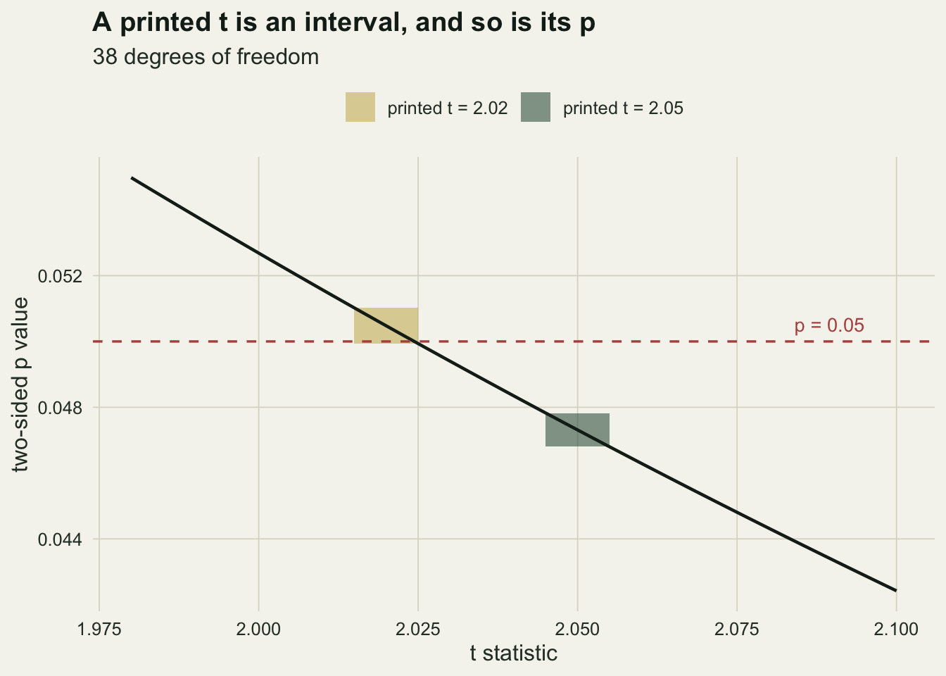

Figure 5: Two-sided p against t with 38 degrees of freedom. Each box spans the rounding interval of a printed t and the p values it allows.

What to report

When a synthesis uses consistency checks, say which ones were run, on which rows, and with which rounding rule. The lenient rule that accepts both neighbours of a tie is the fair default, and at sample sizes that are multiples of eight it gives a different answer from a fixed rule.

Report the number of rows that could be checked, not only the number that failed. GRIM needs integer data, a known number of items per observation and a sample below 10 to the power of the printed decimals; the recomputed p needs a test statistic and its degrees of freedom. A statement that no inconsistencies were found means little if most rows had n above 100.

For each flag, record the most innocent explanation that the arithmetic allows before anything else: the smallest n below the printed one that makes the mean consistent, or the rounding of a statistic near a threshold. Then ask the authors. Brown and Heathers (2017) followed up flagged articles by asking for the data, and Bakker and Wicherts (2011) contacted authors to find where the errors in recomputed p values came from; in both, the printed numbers alone did not settle the matter.

In the extraction sheet, carry the band rather than the point. A mean from 24 nests printed as 3.46 is any value from 3.455 to 3.465 and, from integer data, exactly 83 over 24; a p value recomputed from a printed t is an interval, and an analysis that thresholds it should say which end it used.

Honest limits

GRIM detects endings that no data could produce, and the detection rate computed here assumes those endings are random. Many real errors are not: a transposed pair of digits, a mean copied from the neighbouring column, or a mean with a dropped trailing zero, printed as 3.5 and then checked at one decimal, where n of 10 or more makes the test blind. The closed form describes the grid, not the distribution of mistakes.

Everything here assumes one integer per observation. A mean over several integer items per nest or per respondent is a sum over n times the number of items, which pushes the blind point lower, and a paper that does not say how many items went into a score cannot be checked at all.

The standard deviation check says whether a pair is possible, not whether it is plausible. A printed 1.23 for 20 trees with mean 3.60 would pass, yet it needs 18 trees at 4 and 2 at 0, which may be absurd for defoliation data; no consistency check can say so, because that judgement needs knowledge of the variable. The check also assumes the standard deviation uses n minus one and the same n as the mean. SPRITE goes further by producing candidate samples, and with it the question of which samples are believable.

The p band covers a single t test with integer degrees of freedom. Welch tests print fractional degrees of freedom that are themselves rounded, F and chi squared tests have their own bands, and a one-sided p printed without saying so is half of what a two-sided recomputation gives and will be flagged. statcheck retries a one-sided comparison when the text mentions one-sided testing, and handles several other cases with rules of its own, none of which are tested here.

The false alarm simulation uses one clutch distribution and exclusions at random. Its purpose is to show that one silent exclusion is enough to produce a flag, not to estimate how often papers exclude nests.

References

Brown NJL, Heathers JAJ 2017 Social Psychological and Personality Science 8(4):363-369 (10.1177/1948550616673876)

Nuijten MB, Hartgerink CHJ, van Assen MALM, Epskamp S, Wicherts JM 2016 Behavior Research Methods 48(4):1205-1226 (10.3758/s13428-015-0664-2)

Bakker M, Wicherts JM 2011 Behavior Research Methods 43(3):666-678 (10.3758/s13428-011-0089-5)

Heathers JAJ, Anaya J, van der Zee T, Brown NJL 2018 PeerJ Preprints (10.7287/peerj.preprints.26968v1)

Anaya J 2016 PeerJ Preprints (10.7287/peerj.preprints.2400v1)

Related tutorials

• Effect sizes from incomplete reports
• Rounded and coarsened measurements
• Digit preference and heaping in field data
• Checking for publication bias