library(ggplot2)

te_pal <- list(forest = "#275139", green = "#2f8f63", sage = "#93a87f",
               clay = "#b5534e", gold = "#cda23f", line = "#dad9ca",
               ink = "#16241d", paper = "#f5f4ee")

theme_te <- function() {
  theme_minimal(base_size = 12) +
    theme(panel.grid.minor = element_blank(),
          panel.grid.major = element_line(colour = "#e7e6dc"),
          plot.background = element_rect(fill = "#f5f4ee", colour = NA),
          panel.background = element_rect(fill = "#f5f4ee", colour = NA),
          plot.title = element_text(face = "bold", colour = te_pal$ink),
          axis.title = element_text(colour = "#2c3a31"),
          axis.text = element_text(colour = "#2c3a31"),
          legend.position = "bottom")
}Effect sizes from incomplete reports
R
meta-analysis
effect size
ecology tutorial
Papers print a median and quartiles, not a standard deviation. Measuring what recovered SDs cost an ecological meta-analysis: weights, coverage, bias.
A synthesis of nitrogen addition experiments in temperate grassland: thirty papers published between 1986 and 2021, each with a fertilised plot group and an unfertilised control, each measuring above-ground biomass at peak season. The plan is a random-effects meta-analysis of the log response ratio, the summary Hedges, Gurevitch and Curtis (1999) set out for experimental ecology and the standard one in this literature, and the plan needs two numbers per study: an effect size and its sampling variance.
The papers do not supply them. Reading through the PDFs, some report a mean, a standard deviation and a sample size, which is everything required. Some report a mean and a standard error, which is also everything required as long as you notice which of the two is on the page. Some report a median and an interquartile range, because the biomass data were skewed and a referee asked for a non-parametric summary. A few report nothing but a box plot, from which the median, the quartiles and the whisker ends can be read off the axis with a ruler. Nobody deposited the raw data. Every corresponding author from before 2005 has retired.
This post is about the step before the meta-analysis starts. Five tutorials on this site cover what happens afterwards: random-effects meta-analysis, heterogeneity in meta-analysis, meta-regression with moderators, checking for publication bias and selection models for publication bias. Each of them opens by stating that every study supplies an effect size and a within-study sampling variance that is treated as known. That is the standard textbook framing and there is nothing wrong with it, but no ecologist has ever opened a folder of PDFs and found it true. The publication-bias post is the closest neighbour and it is still a different problem: it is about studies that are missing from the pile, while this one is about statistics that are missing from studies which are sitting in the pile.
What follows measures the cost of filling in the gaps. A corpus of thirty studies is simulated with a known true effect and known heterogeneity, then each study is “published” in one of the four formats above, and the analyst has to reconstruct the effect size and the variance from whatever reached the page. Five things get measured: how accurate the classic recovery formulas are and where each one wins, what a standard error read as a standard deviation does to the weights, whether the weight a study receives is correlated with the error in its recovered standard deviation, which part of the analysis the error lands on for different effect metrics, and what a sensitivity analysis is actually worth.
No meta-analysis package is used. metafor would do all of this correctly and is the right tool for real work, but the formulas here are short enough to write out, and writing them out is the only way to see which term the error enters through.
What the papers actually printed
The generating model is deliberately kind. Each study has a control arm and a treatment arm of the same size, biomass in each arm is normal with a constant coefficient of variation, and the true log response ratio of study \(i\) is drawn from a normal distribution with mean \(\mu\) and between-study standard deviation \(\tau\). Normality matters because every recovery formula below assumes it; giving the formulas skewed data would be a fair test of a different question, and here the point is that they lose accuracy even when their own assumption holds.
k_stud <- 30
mu_true <- 0.25
tau_true <- 0.15
mc_base <- 20
cv_base <- 0.25
z95 <- qnorm(0.975)

arm_summary <- function(x) {
  qq <- unname(quantile(x, c(0.25, 0.75)))
  c(m = mean(x), s = sd(x), med = median(x), q1 = qq[1], q3 = qq[2],
    lo = min(x), hi = max(x))
}

make_corpus <- function(seed, tau_use = tau_true) {
  set.seed(seed)
  n_arm <- sample(8:80, k_stud, replace = TRUE)
  theta <- rnorm(k_stud, mu_true, tau_use)
  rows <- lapply(seq_len(k_stud), function(i) {
    mt <- mc_base * exp(theta[i])
    ac <- arm_summary(rnorm(n_arm[i], mc_base, mc_base * cv_base))
    at <- arm_summary(rnorm(n_arm[i], mt, mt * cv_base))
    names(ac) <- paste0(names(ac), "_c")
    names(at) <- paste0(names(at), "_t")
    c(n_arm = n_arm[i], theta = theta[i], ac, at)
  })
  as.data.frame(do.call(rbind, rows))
}

cp1 <- make_corpus(20260801)
fmt_share <- c("mean and SD" = 12, "mean and SE" = 7,
               "median and IQR" = 7, "median and range" = 4)
cp1$format <- rep(names(fmt_share), fmt_share)
print(fmt_share)
mean and SD mean and SE median and IQR median and range
12 7 7 4 print(round(c(studies = k_stud, smallest_arm = min(cp1$n_arm),
largest_arm = max(cp1$n_arm), median_arm = median(cp1$n_arm),
true_lnrr = mu_true, true_tau = tau_true), 3)) studies smallest_arm largest_arm median_arm true_lnrr true_tau
30.00 8.00 80.00 47.50 0.25 0.15 Thirty studies, arms from 8 to 80 plants with a median of 47.5, a true mean log response ratio of 0.25 (a 28.4 per cent increase in biomass) and a between-study standard deviation of 0.15. The report formats are assigned in the proportions above: 12 studies give the analyst everything, 7 give a mean and a standard error, and 11 give a median with either quartiles or a range. So 18 of 30 studies, 60 per cent of the corpus, need something done to them before they can enter a weighted average.
Here is what one study of each kind puts on the page, for the treatment arm.
as_printed <- function(i) {
  rw <- cp1[i, ]
  spread <- switch(rw$format,
    "mean and SD" = sprintf("SD %.2f", rw$s_t),
    "mean and SE" = sprintf("SE %.2f", rw$s_t / sqrt(rw$n_arm)),
    "median and IQR" = sprintf("Q1 %.2f, Q3 %.2f", rw$q1_t, rw$q3_t),
    "median and range" = sprintf("min %.2f, max %.2f", rw$lo_t, rw$hi_t))
  centre <- if (rw$format %in% c("mean and SD", "mean and SE"))
    sprintf("mean %.2f", rw$m_t) else sprintf("median %.2f", rw$med_t)
  data.frame(format = rw$format, n = rw$n_arm, centre = centre, spread = spread)
}
one_each <- vapply(names(fmt_share), function(f) which(cp1$format == f)[1], integer(1))
print(do.call(rbind, lapply(one_each, as_printed)), row.names = FALSE)
format n centre spread
mean and SD 28 mean 25.67 SD 6.93
mean and SE 40 mean 24.08 SE 0.76
median and IQR 56 median 31.03 Q1 25.74, Q3 34.97
median and range 26 median 23.40 min 15.17, max 32.06The first row is complete. The second is complete too, provided the reader multiplies by the square root of the sample size rather than taking the number at face value. The third and fourth rows contain no standard deviation at all, and no arithmetic recovers one exactly. What they contain is enough information to make a normal-theory guess at it, and the literature has several such guesses. Weir et al (2018) catalogue the ones in circulation and how often each of them is reached for.
Recovering a standard deviation from a median
Two families of formula are in common use. Hozo, Djulbegovic and Hozo (2005) work from the minimum, the median, the maximum and the sample size, with three cases: a closed form for \(n \le 15\), the range divided by four for \(15 < n \le 70\), and the range divided by six above that. Wan, Wang, Liu and Tong (2014) replace the piecewise constants with the expected value of the relevant order statistic under normality, which gives a smooth function of \(n\) for the range-based case and a second formula for the case where quartiles are printed instead. The fourth candidate is the rule of thumb every referee has seen, the interquartile range divided by 1.349, which is the large-sample limit of Wan’s quartile formula with no correction for sample size. Hozo’s paper and Wan’s each also supply a formula for the arm mean itself, and those two are what the code below uses for it; Luo et al (2018) improve on both by weighting the printed statistics according to the sample size.
sd_hozo <- function(lo, med, hi, nn) {
  if (nn <= 15) sqrt((((lo - 2 * med + hi)^2) / 4 + (hi - lo)^2) / 12)
  else if (nn <= 70) (hi - lo) / 4
  else (hi - lo) / 6
}
sd_wan_rng <- function(lo, hi, nn)
  (hi - lo) / (2 * qnorm((nn - 0.375) / (nn + 0.25)))
sd_wan_iqr <- function(q1, q3, nn)
  (q3 - q1) / (2 * qnorm((0.75 * nn - 0.125) / (nn + 0.25)))
sd_rule <- function(q1, q3) (q3 - q1) / 1.349
Each estimator is applied to 3,000 normal samples at five arm sizes, with a true standard deviation of five units. Relative bias and relative root mean squared error are both reported as percentages of that true value, because the error that matters downstream is proportional rather than absolute.
set.seed(20260802)
n_draw <- 3000
n_grid <- c(10, 20, 40, 80, 160)
sd_ref <- 5
meth_lab <- c("Hozo range", "Wan range", "Wan IQR", "IQR over 1.349")
rec <- do.call(rbind, lapply(n_grid, function(nn) {
  err <- matrix(NA_real_, n_draw, 4)
  m_err <- matrix(NA_real_, n_draw, 2)
  for (r in seq_len(n_draw)) {
    a <- arm_summary(rnorm(nn, 20, sd_ref))
    err[r, ] <- c(sd_hozo(a[["lo"]], a[["med"]], a[["hi"]], nn),
                  sd_wan_rng(a[["lo"]], a[["hi"]], nn),
                  sd_wan_iqr(a[["q1"]], a[["q3"]], nn),
                  sd_rule(a[["q1"]], a[["q3"]])) - sd_ref
    m_err[r, ] <- c((a[["lo"]] + 2 * a[["med"]] + a[["hi"]]) / 4,
                    (a[["q1"]] + a[["med"]] + a[["q3"]]) / 3) - 20
  }
  data.frame(n_arm = nn, method = meth_lab,
             rel_bias = 100 * colMeans(err) / sd_ref,
             rel_rmse = 100 * sqrt(colMeans(err^2)) / sd_ref,
             mean_rmse_rng = 100 * sqrt(mean(m_err[, 1]^2)) / 20,
             mean_rmse_iqr = 100 * sqrt(mean(m_err[, 2]^2)) / 20)
}))
print(round(rec[, c("n_arm", "rel_bias", "rel_rmse")], 3))
n_arm rel_bias rel_rmse
1 10 -10.386 25.399
2 10 -0.620 25.704
3 10 0.563 36.737
4 10 -13.318 34.350
5 20 -6.817 19.442
6 20 -0.245 19.493
7 20 0.505 26.424
8 20 -6.619 25.423
9 40 7.422 17.890
10 40 -0.368 15.102
11 40 0.292 18.102
12 40 -3.313 17.760
13 80 -18.978 21.573
14 80 0.495 12.732
15 80 -0.130 12.996
16 80 -1.938 12.906
17 160 -10.892 14.643
18 160 0.476 11.047
19 160 -0.139 8.988
20 160 -1.047 8.966print(rec$method[1:4])[1] "Hozo range" "Wan range" "Wan IQR" "IQR over 1.349"gv <- function(nn, mth, col) rec[[col]][rec$n_arm == nn & rec$method == mth]
gap_rng_iqr <- vapply(n_grid, function(nn)
gv(nn, "Wan range", "rel_rmse") - gv(nn, "Wan IQR", "rel_rmse"), numeric(1))
print(round(rbind(n_arm = n_grid, range_minus_iqr_rmse = gap_rng_iqr), 4)) [,1] [,2] [,3] [,4] [,5]
n_arm 10.0000 20.0000 40.0000 80.0000 160.000
range_minus_iqr_rmse -11.0333 -6.9314 -2.9993 -0.2635 2.059print(round(c(mean_rmse_from_range = rec$mean_rmse_rng[rec$n_arm == 40][1],
mean_rmse_from_iqr = rec$mean_rmse_iqr[rec$n_arm == 40][1],
sd_rmse_from_iqr = gv(40, "Wan IQR", "rel_rmse")), 3))mean_rmse_from_range mean_rmse_from_iqr sd_rmse_from_iqr
5.282 4.249 18.102 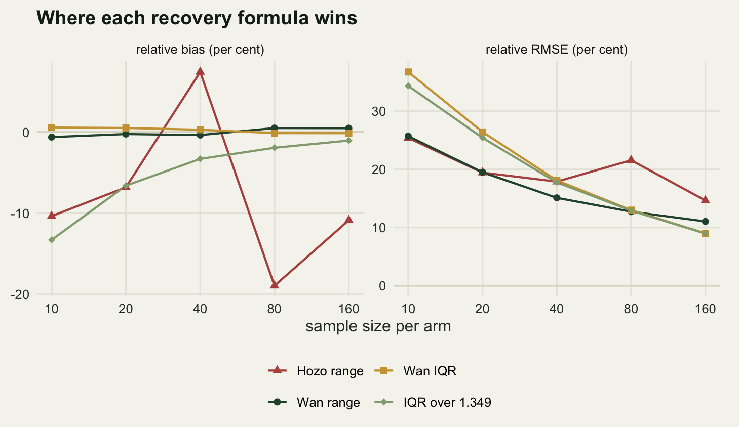
Hozo’s estimator is the only one whose bias stays large at every arm size tested, and the shape of its bias is a direct print of its own cut points. At an arm of 40 it runs 7.42 per cent high, because the range divided by four is too generous there. At an arm of 80, just past the cut at 70 where the divisor changes from four to six, it runs 18.98 per cent low. The sign turns over inside that branch: at an arm of 20 the same range divided by four runs 6.82 per cent low. A meta-analysis whose studies straddle the cut therefore receives standard deviations whose error changes sign with sample size, not simply too large below the cut and too small above it. The paper is twenty years old and has been superseded, but it remains the formula most often cited in ecological reviews, so the pattern is worth recognising.
The two Wan estimators are close to unbiased at every arm size tested, the largest deviation being 0.62 per cent. Their precision crosses over. At an arm of 10 the range-based version has a relative RMSE of 25.7 per cent against 36.74 per cent for the quartile version, so the range wins by 11.03 percentage points. By an arm of 160 the order has reversed, 11.05 against 8.99 per cent. The crossing is just above an arm of 80, where the two differ by 0.26 percentage points.
The reason is that the two extremes carry a great deal of information about the spread when there are ten observations and almost none when there are one hundred and sixty, at which point they are two draws from the tails and the quartiles are estimated from dozens of points each. So the practical rule is the opposite of the intuitive one: prefer a printed range in small studies, prefer printed quartiles in large ones, and do not treat “more extreme statistics” as “more information”. The naive interquartile rule tracks Wan’s quartile formula closely once the arm passes 40 and is 13.32 per cent low at an arm of 10, which is the small-sample correction earning its place.
One number puts the whole exercise in proportion. At an arm of 40, recovering the mean from a median and quartiles has a relative RMSE of 4.25 per cent, while recovering the standard deviation from the same three numbers has a relative RMSE of 18.1 per cent, about 4.3 times worse. The centre of a distribution survives summarisation; the spread does not. That asymmetry decides which part of a meta-analysis is damaged, and the section after next takes it apart.
A standard error read as a standard deviation
Before any of the recovery formulas matter, there is a plainer error to price. A paper prints a mean, a plus-or-minus sign and a second number, and never says what the second number is. Reading a standard error as a standard deviation is the single most common mistake in this part of the workflow, and unlike an imprecise recovery it is not noise: it understates the spread by a factor of the square root of the sample size, every time, in the same direction.
For the log response ratio the effect size depends only on the two arm means, so a wrong standard deviation does not move it at all. That holds for the plain estimator used here; Lajeunesse (2015) derives a small-sample correction to it which does read the standard deviations, and under that version a recovery error would reach the effect size after all. A wrong standard deviation moves the sampling variance, and through that the weight:
\[v_i = \frac{s_{c,i}^2}{n_i \bar{x}_{c,i}^2} + \frac{s_{t,i}^2}{n_i \bar{x}_{t,i}^2}\]
Substituting \(s/\sqrt{n}\) for \(s\) divides both terms by \(n_i\), so the variance is exactly \(n_i\) times too small and the study’s unnormalised inverse-variance weight is exactly \(n_i\) times too large. Not approximately: exactly, and by an amount that grows with the size of the study.
lnrr_of <- function(cp) log(cp$m_t / cp$m_c)
v_lnrr <- function(cp, s_c, s_t)
  s_c^2 / (cp$n_arm * cp$m_c^2) + s_t^2 / (cp$n_arm * cp$m_t^2)

pool_re <- function(y, v) {
  wt <- 1 / v
  mu_f <- sum(wt * y) / sum(wt)
  q_stat <- sum(wt * (y - mu_f)^2)
  cc <- sum(wt) - sum(wt^2) / sum(wt)
  t2 <- max(0, (q_stat - (length(y) - 1)) / cc)
  ws <- 1 / (v + t2)
  c(mu = sum(ws * y) / sum(ws), se = sqrt(1 / sum(ws)), tau2 = t2,
    i2 = max(0, (q_stat - (length(y) - 1)) / q_stat),
    mu_fe = mu_f, se_fe = sqrt(1 / sum(wt)))
}

mis_idx <- which(cp1$format == "mean and SE")
sb_c <- cp1$s_c
sb_t <- cp1$s_t
sb_c[mis_idx] <- cp1$s_c[mis_idx] / sqrt(cp1$n_arm[mis_idx])
sb_t[mis_idx] <- cp1$s_t[mis_idx] / sqrt(cp1$n_arm[mis_idx])
v_ok <- v_lnrr(cp1, cp1$s_c, cp1$s_t)
v_bad <- v_lnrr(cp1, sb_c, sb_t)
w_ok <- (1 / v_ok) / sum(1 / v_ok)
w_bad <- (1 / v_bad) / sum(1 / v_bad)
keff <- function(w) 1 / sum(w^2)

print(round(c(raw_inflation_max_gap = max(abs((v_ok / v_bad)[mis_idx] -
                                                cp1$n_arm[mis_idx])),
              share_ok = sum(w_ok[mis_idx]), share_bad = sum(w_bad[mis_idx]),
              largest_single_share_ok = max(w_ok),
              largest_single_share_bad = max(w_bad),
              keff_ok = keff(w_ok), keff_bad = keff(w_bad)), 5))
raw_inflation_max_gap share_ok share_bad
0.00000 0.30738 0.96440
largest_single_share_ok largest_single_share_bad keff_ok
0.07838 0.31025 22.76174
keff_bad
5.49034 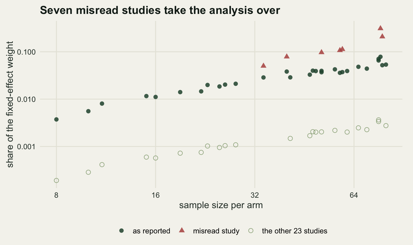
In the display corpus the ratio of correct to misread sampling variance equals the arm size to within 0, confirming the algebra. The consequence is that 7 studies which should hold 30.7 per cent of the fixed-effect weight end up holding 96.4 per cent of it. One study alone goes from 7.8 per cent to 31 per cent. The effective number of studies contributing, computed as the inverse of the sum of squared weights, falls from 22.76 to 5.49 out of 30.
That is one corpus. The next block repeats it over eight hundred corpora at two levels of between-study heterogeneity: none at all, and the 0.15 used throughout. Both a fixed-effect and a DerSimonian-Laird random-effects pooling are computed each time, along with the coverage of a nominal 95 per cent interval for the true mean.
run_mis <- function(tau_use, seed0, n_rep = 800) {
  acc <- numeric(16)
  keep <- matrix(NA_real_, n_rep, 8)
  for (r in seq_len(n_rep)) {
    cp <- make_corpus(seed0 + r, tau_use = tau_use)
    y <- lnrr_of(cp)
    mis <- mis_idx
    bc <- cp$s_c
    bt <- cp$s_t
    bc[mis] <- cp$s_c[mis] / sqrt(cp$n_arm[mis])
    bt[mis] <- cp$s_t[mis] / sqrt(cp$n_arm[mis])
    vA <- v_lnrr(cp, cp$s_c, cp$s_t)
    vB <- v_lnrr(cp, bc, bt)
    pA <- pool_re(y, vA)
    pB <- pool_re(y, vB)
    wA <- (1 / vA) / sum(1 / vA)
    wB <- (1 / vB) / sum(1 / vB)
    acc <- acc + c(pA[["mu_fe"]], pA[["se_fe"]], pA[["mu"]], pA[["se"]],
                   pA[["tau2"]], pA[["i2"]],
                   pB[["mu_fe"]], pB[["se_fe"]], pB[["mu"]], pB[["se"]],
                   pB[["tau2"]], pB[["i2"]],
                   sum(wA[mis]), sum(wB[mis]), keff(wA), keff(wB))
    keep[r, ] <- c(pA[["mu_fe"]], pB[["mu_fe"]], pA[["mu"]], pB[["mu"]],
                   pA[["se_fe"]], pB[["se_fe"]], pA[["se"]], pB[["se"]])
  }
  acc <- acc / n_rep
  names(acc) <- c("fe_mu", "fe_se", "re_mu", "re_se", "tau2", "i2",
                  "fe_mu_x", "fe_se_x", "re_mu_x", "re_se_x", "tau2_x", "i2_x",
                  "wshare", "wshare_x", "keff", "keff_x")
  cover <- function(v, s) mean(abs(v - mu_true) < z95 * s)
  c(acc, reps = n_rep,
    fe_cov = cover(keep[, 1], keep[, 5]),
    fe_cov_x = cover(keep[, 2], keep[, 6]),
    re_cov = cover(keep[, 3], keep[, 7]),
    re_cov_x = cover(keep[, 4], keep[, 8]),
    fe_sd = sd(keep[, 1]), fe_sd_x = sd(keep[, 2]),
    re_sd = sd(keep[, 3]), re_sd_x = sd(keep[, 4]))
}
mis0 <- run_mis(0, 20261000)
mis15 <- run_mis(tau_true, 20263000)
print(round(mis0, 5))
fe_mu fe_se re_mu re_se tau2 i2 fe_mu_x fe_se_x
0.25029 0.00966 0.25029 0.01032 0.00036 0.09214 0.25047 0.00273
re_mu_x re_se_x tau2_x i2_x wshare wshare_x keff keff_x
0.25003 0.01145 0.00230 0.85245 0.23333 0.93691 24.18758 5.07353
reps fe_cov fe_cov_x re_cov re_cov_x fe_sd fe_sd_x re_sd
800.00000 0.93000 0.20875 0.94500 0.91625 0.01023 0.02117 0.01025
re_sd_x
0.01193 print(round(mis15, 5)) fe_mu fe_se re_mu re_se tau2 i2 fe_mu_x fe_se_x
0.25033 0.00966 0.25047 0.02940 0.02268 0.87917 0.25368 0.00273
re_mu_x re_se_x tau2_x i2_x wshare wshare_x keff keff_x
0.25047 0.02906 0.02474 0.98310 0.23343 0.93679 24.16427 5.11506
reps fe_cov fe_cov_x re_cov re_cov_x fe_sd fe_sd_x re_sd
800.00000 0.44250 0.04000 0.94625 0.90875 0.03121 0.06978 0.02957
re_sd_x
0.02952 Take the homogeneous corpus first, where a fixed-effect analysis is the correct model. Read correctly, it returns a mean standard error of 0.00966 against an actual spread of estimates of 0.01023, and covers the truth 93 per cent of the time. Read wrongly, the reported standard error falls to 0.00273, a factor of 3.54 narrower, while the actual spread of the estimates rises to 0.02117, a factor of 2.07 wider. Coverage goes from 93 per cent to 20.9 per cent. The pooled estimate itself barely moves, 0.2503 against 0.2505, because the misread studies are not selected for their results. The failure is entirely in the interval, and an interval that covers the truth 20.9 per cent of the time is worse than no interval at all, because it will be believed.
The random-effects fit is where this gets interesting, and where it goes against what I expected before running it. Under the same misreading, random-effects coverage moves only from 94.5 per cent to 91.6 per cent. The model absorbs the damage. It absorbs it by inventing between-study variance: with correct standard errors and a genuinely homogeneous corpus, the estimated tau-squared is 0.00036 and I-squared is 9.2 per cent, which is the right answer. With the misreading, tau-squared becomes 0.0023 and I-squared becomes 85.2 per cent.
That number deserves a sentence on its own. Seven papers whose error bars were labelled ambiguously produce an I-squared of 85.2 per cent in a set of studies that all estimate exactly the same effect. Cochran’s Q does not know the difference between studies that genuinely disagree and studies whose claimed precision is a fiction; it only sees observations further from the weighted mean than their stated variances allow. Everything the heterogeneity tutorial teaches you to report, and everything a reader would conclude from it about context dependence in the ecology, is downstream of a units error.
At the realistic heterogeneity of 0.15 the same pattern holds with the numbers moved along. Fixed-effect coverage falls from 44.2 per cent to 4 per cent, random-effects coverage from 94.6 to 90.9 per cent, and I-squared is pushed from an already high 87.9 per cent to 98.3 per cent, where it stops being able to say anything at all. The effective number of contributing studies is 5.12 against 24.16.
The weight is correlated with the recovery error
Now the quieter case: no misreading, just recovery. Wan’s quartile formula is applied to every study in each simulated corpus, not only to the ones whose printed format would have forced it, and the arm means are left alone, so the whole weight change is down to the recovered standard deviation. The mean recovery enters later, in the sweeps that follow. Those recovered standard deviations are close to unbiased, as the second section showed, so it is tempting to treat them as adding noise and nothing else.
They do not, because of where the recovered value enters. The weight is one over a variance, and a variance is the square of the recovered standard deviation, so the map from recovery error to weight is decreasing and convex. A study whose standard deviation came out too small receives more weight than it should, and the studies which received the most weight are therefore, on average, the ones whose spread was most understated.
set.seed(20265000)
cor_dat <- do.call(rbind, lapply(seq_len(10), function(j) {
  cp <- make_corpus(20265100 + j)
  shc <- sd_wan_iqr(cp$q1_c, cp$q3_c, cp$n_arm)
  sht <- sd_wan_iqr(cp$q1_t, cp$q3_t, cp$n_arm)
  v_tru <- v_lnrr(cp, cp$s_c, cp$s_t)
  v_hat <- v_lnrr(cp, shc, sht)
  data.frame(sd_err = 100 * (shc - cp$s_c) / cp$s_c,
             w_change = 100 * ((1 / v_hat) / sum(1 / v_hat) -
                                 (1 / v_tru) / sum(1 / v_tru)))
}))
w_fit <- lm(w_change ~ sd_err, data = cor_dat)
print(round(c(n_points = nrow(cor_dat),
              correlation = cor(cor_dat$sd_err, cor_dat$w_change),
              slope = unname(coef(w_fit)[2]),
              slope_se = summary(w_fit)$coefficients[2, 2],
              p_value = summary(w_fit)$coefficients[2, 4]), 6))
n_points correlation slope slope_se p_value
300.000000 -0.590131 -0.024307 0.001926 0.000000 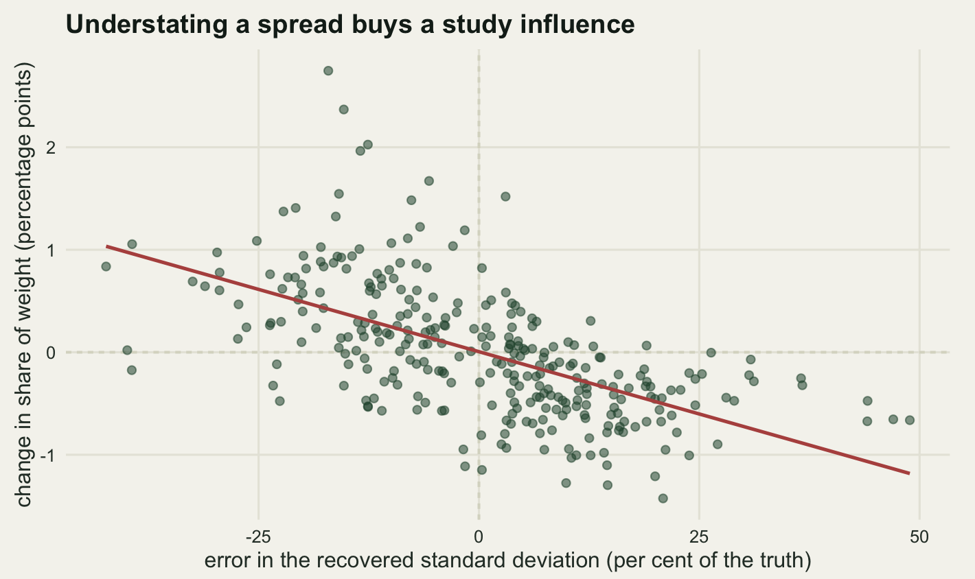
Over 300 studies the correlation is -0.5901, with a fitted slope of -0.02431 percentage points of weight per percentage point of standard deviation error and a standard error of 0.00193. The correlation is there and it is not small, which is what I expected before running any of this.
The question is what it costs. The next sweep crosses four imputation fractions with four levels of true between-study heterogeneity, refits the random-effects model each time, and records the pooled estimate, the interval width and the coverage. Because every fraction is evaluated on the same corpus, the shift caused by imputation can be measured as a paired difference, which is far more precise than comparing two independent averages.
tau_grid <- c(0, 0.05, 0.10, 0.20)
fr_grid <- c(0, 0.3, 0.6, 1)
n_repd <- 1200
sweep_rows <- list()
paired <- list()
for (tg in tau_grid) {
  acc <- matrix(0, length(fr_grid), 5)
  pair_mu <- matrix(NA_real_, n_repd, 2)
  for (r in seq_len(n_repd)) {
    cp <- make_corpus(20267000 + r, tau_use = tg)
    ord <- sample.int(k_stud)
    shc <- sd_wan_iqr(cp$q1_c, cp$q3_c, cp$n_arm)
    sht <- sd_wan_iqr(cp$q1_t, cp$q3_t, cp$n_arm)
    mhc <- (cp$q1_c + cp$med_c + cp$q3_c) / 3
    mht <- (cp$q1_t + cp$med_t + cp$q3_t) / 3
    for (j in seq_along(fr_grid)) {
      idx <- ord[seq_len(round(fr_grid[j] * k_stud))]
      s_c <- cp$s_c
      s_t <- cp$s_t
      cp2 <- cp
      if (length(idx)) {
        s_c[idx] <- shc[idx]
        s_t[idx] <- sht[idx]
        cp2$m_c[idx] <- mhc[idx]
        cp2$m_t[idx] <- mht[idx]
      }
      pp <- pool_re(lnrr_of(cp2), v_lnrr(cp2, s_c, s_t))
      acc[j, ] <- acc[j, ] + c(pp[["mu"]], pp[["se"]], pp[["tau2"]],
                               abs(pp[["mu"]] - mu_true) < z95 * pp[["se"]],
                               pp[["mu"]]^2)
      if (j == 1) pair_mu[r, 1] <- pp[["mu"]]
      if (j == length(fr_grid)) pair_mu[r, 2] <- pp[["mu"]]
    }
  }
  acc <- acc / n_repd
  sweep_rows[[length(sweep_rows) + 1]] <- data.frame(
    tau = tg, frac = fr_grid, mu = acc[, 1], se = acc[, 2], tau2 = acc[, 3],
    coverage = acc[, 4], sd_mu = sqrt(pmax(0, acc[, 5] - acc[, 1]^2)))
  dif <- pair_mu[, 2] - pair_mu[, 1]
  paired[[length(paired) + 1]] <- data.frame(
    tau = tg, mean_shift = mean(dif), shift_mc_se = sd(dif) / sqrt(n_repd),
    sd_of_shift = sd(dif))
}
sw <- do.call(rbind, sweep_rows)
sw$width <- 2 * z95 * sw$se
sw$bias <- sw$mu - mu_true
pr <- do.call(rbind, paired)
cov_bar <- mean(sw$coverage)
cov_mc_se <- sqrt(cov_bar * (1 - cov_bar) / n_repd)
print(round(sw, 5))
tau frac mu se tau2 coverage sd_mu width bias
1 0.00 0.0 0.24965 0.01026 0.00032 0.96833 0.00945 0.04023 -0.00035
2 0.00 0.3 0.24965 0.01041 0.00041 0.96083 0.00978 0.04079 -0.00035
3 0.00 0.6 0.24965 0.01055 0.00049 0.95583 0.01007 0.04137 -0.00035
4 0.00 1.0 0.24966 0.01079 0.00063 0.95917 0.01024 0.04231 -0.00034
5 0.05 0.0 0.25037 0.01378 0.00265 0.94583 0.01372 0.05402 0.00037
6 0.05 0.3 0.25032 0.01398 0.00280 0.94583 0.01382 0.05480 0.00032
7 0.05 0.6 0.25031 0.01417 0.00293 0.94250 0.01408 0.05554 0.00031
8 0.05 1.0 0.25044 0.01442 0.00312 0.94667 0.01436 0.05652 0.00044
9 0.10 0.0 0.25042 0.02118 0.01016 0.95167 0.02117 0.08301 0.00042
10 0.10 0.3 0.25038 0.02132 0.01031 0.94667 0.02118 0.08356 0.00038
11 0.10 0.6 0.25035 0.02145 0.01045 0.95000 0.02141 0.08409 0.00035
12 0.10 1.0 0.25044 0.02163 0.01065 0.95083 0.02162 0.08480 0.00044
13 0.20 0.0 0.25041 0.03795 0.04019 0.94167 0.03797 0.14875 0.00041
14 0.20 0.3 0.25038 0.03804 0.04033 0.94583 0.03793 0.14910 0.00038
15 0.20 0.6 0.25035 0.03812 0.04046 0.94583 0.03814 0.14943 0.00035
16 0.20 1.0 0.25041 0.03824 0.04067 0.94750 0.03827 0.14989 0.00041print(round(pr, 6)) tau mean_shift shift_mc_se sd_of_shift
1 0.00 7.0e-06 0.000123 0.004244
2 0.05 7.2e-05 0.000127 0.004383
3 0.10 2.1e-05 0.000127 0.004388
4 0.20 0.0e+00 0.000128 0.004442print(round(c(coverage_mc_se = cov_mc_se, replicates = n_repd), 5))coverage_mc_se replicates
6.27e-03 1.20e+03 qs <- function(tg, fr, col) sw[[col]][sw$tau == tg & sw$frac == fr]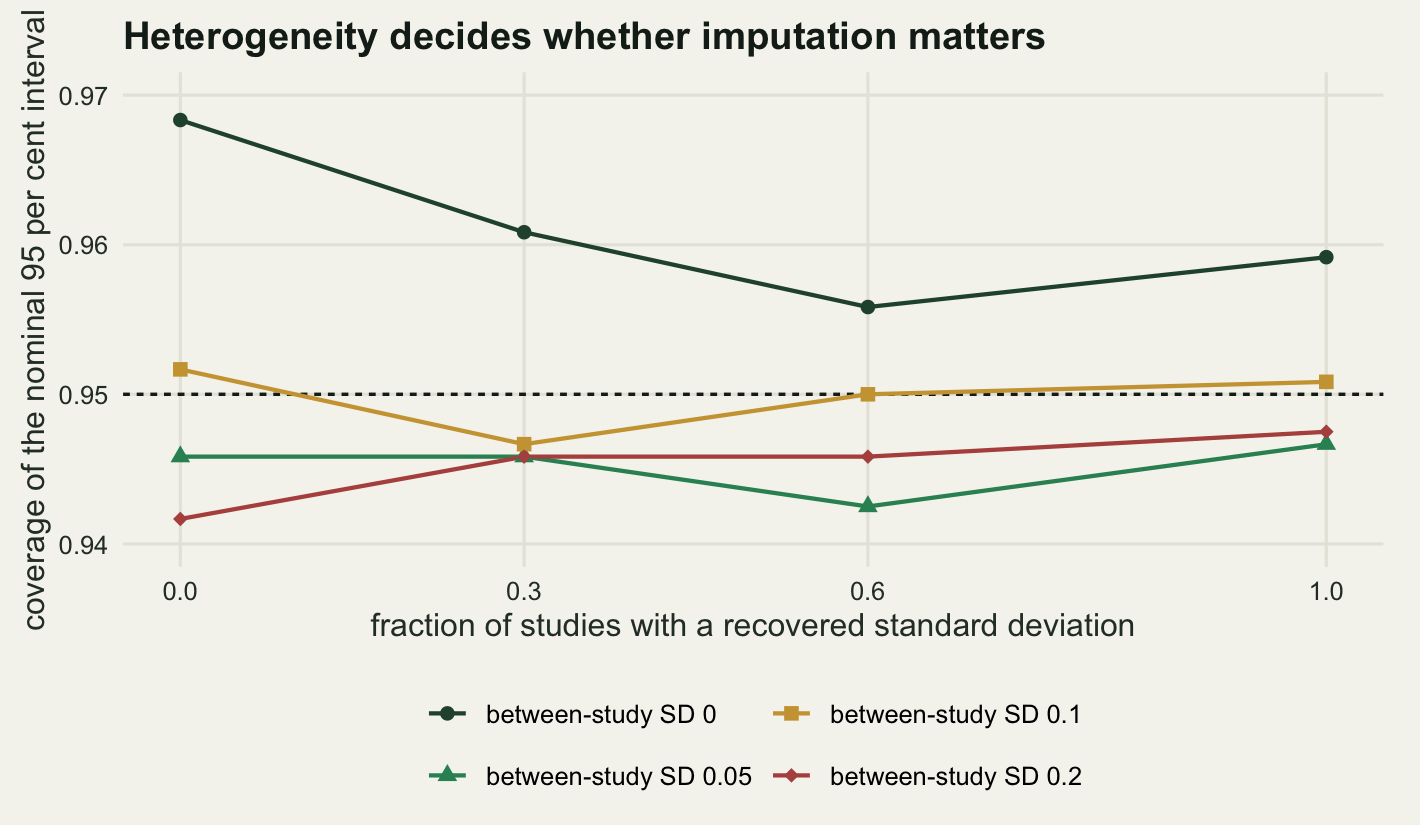
This is the part that did not come out the way I expected, and the numbers are clear enough to say so plainly. Going from no imputation to every study imputed, in the homogeneous corpus, the reported interval widens from 0.04023 to 0.04231, a rise of 5.17 per cent, while the actual spread of the pooled estimate rises from 0.00945 to 0.01024, a rise of 8.34 per cent. The spread does outgrow the interval, which is the predicted direction, and coverage duly falls from 96.8 per cent to 95.9 per cent. But the Monte Carlo standard error on a coverage estimate from 1200 replicates is 0.63 percentage points, so a fall of 0.92 points is at the edge of what this many replicates can resolve. The honest summary is that imputing every standard deviation in a homogeneous corpus costs on the order of one point of coverage, and that the interval had a point to spare: at a true between-study standard deviation of zero the DerSimonian-Laird estimator is truncated at a boundary it wants to sit on, so the interval starts out conservative at 96.8 per cent rather than at 95.
At the three positive levels of heterogeneity the imputation costs nothing detectable. At a between-study standard deviation of 0.2 the interval widens by only 0.77 per cent from no imputation to full imputation, against 5.17 per cent in the homogeneous case, and coverage ends where it started.
The paired shifts settle the question of direction with more precision than coverage can. Imputing every study rather than none moves the pooled estimate by 6.84e-06 in the homogeneous corpus and by -4.76e-07 at a between-study standard deviation of 0.2, against Monte Carlo standard errors of 1.23e-04 and 1.28e-04. Both shifts are smaller than their own Monte Carlo standard error, on a true effect of 0.25. Whatever the correlated weights are doing, they are not producing a directional bias of a size that would appear in a results section.
The mechanism explains the anticlimax. Inverse-variance weighting is insensitive to weight error in two separate ways. Averaging over thirty studies cancels most of an unbiased recovery error, since the studies whose spread was understated are balanced by those whose spread was overstated. And once tau-squared is added to every within-study variance, it dominates the denominator, so the weights flatten towards equality and stop caring what the within-study variances were. Between-study heterogeneity, which the sibling tutorials treat as the problem, is the thing protecting the pooled estimate here. The correlation of -0.59 is real and it is the right mechanism to worry about; what it is not is a large source of error in a pooled mean, and the difference between those two statements is the difference between a diagnostic worth running and a finding worth reporting.
The contrast with the previous section is the point. A recovery error of 18.1 per cent, unbiased and independent across studies, is almost free. A units error that scales every affected variance by the same power of the same quantity is not, because nothing cancels it.
Where the damage lands depends on the effect metric
The log response ratio has a property that made the last two sections possible: the effect size uses only the arm means, so a wrong standard deviation cannot touch it. Hedges’ g, which the random-effects tutorial uses and which is the other common ecological metric, is the reverse. It divides the mean difference by the pooled standard deviation, so a recovery error goes straight into the effect size, and its sampling variance depends on the standard deviation only weakly, through the squared effect size.
g_of <- function(cp, s_c, s_t) {
  spool <- sqrt(((cp$n_arm - 1) * s_c^2 + (cp$n_arm - 1) * s_t^2) /
                  (2 * cp$n_arm - 2))
  dd <- (cp$m_t - cp$m_c) / spool
  jj <- 1 - 3 / (4 * (2 * cp$n_arm - 2) - 1)
  cbind(g = jj * dd, v = jj^2 * (2 / cp$n_arm + dd^2 / (4 * cp$n_arm)))
}

n_repg <- 800
accg <- numeric(6)
for (r in seq_len(n_repg)) {
  cp <- make_corpus(20269000 + r)
  shc <- sd_wan_iqr(cp$q1_c, cp$q3_c, cp$n_arm)
  sht <- sd_wan_iqr(cp$q1_t, cp$q3_t, cp$n_arm)
  gt <- g_of(cp, cp$s_c, cp$s_t)
  gh <- g_of(cp, shc, sht)
  wg_t <- (1 / gt[, 2]) / sum(1 / gt[, 2])
  wg_h <- (1 / gh[, 2]) / sum(1 / gh[, 2])
  vl_t <- v_lnrr(cp, cp$s_c, cp$s_t)
  vl_h <- v_lnrr(cp, shc, sht)
  wl_t <- (1 / vl_t) / sum(1 / vl_t)
  wl_h <- (1 / vl_h) / sum(1 / vl_h)
  accg <- accg + c(mean(abs(shc - cp$s_c) / cp$s_c),
                   mean(abs(gh[, 1] - gt[, 1])) / mean(abs(gt[, 1])),
                   mean(abs(wg_h - wg_t)) / mean(wg_t),
                   0,
                   mean(abs(wl_h - wl_t)) / mean(wl_t),
                   pool_re(gh[, 1], gh[, 2])[["mu"]] /
                     pool_re(gt[, 1], gt[, 2])[["mu"]])
}
accg <- accg / n_repg
names(accg) <- c("sd_error", "g_effect_shift", "g_weight_shift",
                 "lnrr_effect_shift", "lnrr_weight_shift", "pooled_g_ratio")
print(round(100 * accg, 4))
sd_error g_effect_shift g_weight_shift lnrr_effect_shift
12.5856 9.3399 1.9558 0.0000
lnrr_weight_shift pooled_g_ratio
15.2131 99.8268 The standard deviations here are wrong by 12.59 per cent on average, and the two metrics route that error to opposite places. For Hedges’ g the per-study effect size moves by 9.34 per cent of its own magnitude while the weight moves by 1.96 per cent. For the log response ratio the effect size moves by exactly 0 per cent, since it never saw the standard deviation, while the weight moves by 15.21 per cent.
Both routes are survivable in a pooled mean of thirty studies: the pooled g comes out at 99.83 per cent of its correct value. But the two failures behave differently everywhere else. Effect-size error propagates into a forest plot, into a funnel plot, into any moderator analysis, and into the between-study variance, because all of those read the individual effect sizes. Weight error stays inside the pooling arithmetic. Choosing the log response ratio when the standard deviations had to be recovered therefore quarantines the damage in the one place where averaging is most likely to absorb it, which is a reason to prefer it that has nothing to do with the usual argument about interpretability.
A sensitivity analysis, and what it is worth
The standard advice is to refit with the imputed studies handled differently and report how far the conclusion moves. Two versions are common: drop them, or keep them with their variances inflated to acknowledge that they were guessed. Wiebe et al (2006) went through the published record and found no agreed way of doing either, or of reporting that it had been done. The block below runs both versions against the full analysis and against the unobtainable complete-report analysis, on a corpus where most of the standard deviations had to be recovered.
sens_frac <- 0.6
sens_infl <- 2

run_sens <- function(tau_use, seed0, frac = sens_frac, infl = sens_infl,
                     n_rep = 800) {
  m_imp <- round(frac * k_stud)
  acc <- matrix(0, 4, 3)
  spread <- numeric(n_rep)
  movecw <- numeric(n_rep)
  contains <- 0
  for (r in seq_len(n_rep)) {
    cp <- make_corpus(seed0 + r, tau_use = tau_use)
    idx <- sample.int(k_stud, m_imp)
    shc <- sd_wan_iqr(cp$q1_c, cp$q3_c, cp$n_arm)
    sht <- sd_wan_iqr(cp$q1_t, cp$q3_t, cp$n_arm)
    cp2 <- cp
    cp2$m_c[idx] <- ((cp$q1_c + cp$med_c + cp$q3_c) / 3)[idx]
    cp2$m_t[idx] <- ((cp$q1_t + cp$med_t + cp$q3_t) / 3)[idx]
    s_c <- cp$s_c
    s_t <- cp$s_t
    s_c[idx] <- shc[idx]
    s_t[idx] <- sht[idx]
    yy <- lnrr_of(cp2)
    vv <- v_lnrr(cp2, s_c, s_t)
    vd <- vv
    vd[idx] <- vd[idx] * infl
    kp <- setdiff(seq_len(k_stud), idx)
    fits <- list(pool_re(lnrr_of(cp), v_lnrr(cp, cp$s_c, cp$s_t)),
                 pool_re(yy, vv), pool_re(yy, vd),
                 pool_re(yy[kp], vv[kp]))
    for (j in 1:4) acc[j, ] <- acc[j, ] +
      c(fits[[j]][["mu"]], fits[[j]][["se"]],
        abs(fits[[j]][["mu"]] - mu_true) < z95 * fits[[j]][["se"]])
    three <- vapply(fits[2:4], function(z) z[["mu"]], numeric(1))
    spread[r] <- max(three) - min(three)
    if (mu_true >= min(three) && mu_true <= max(three)) contains <- contains + 1
    movecw[r] <- abs(three[3] - three[1]) / (z95 * fits[[2]][["se"]])
  }
  acc <- acc / n_rep
  dimnames(acc) <- list(c("complete report", "imputed", "imputed down-weighted",
                          "imputed dropped"), c("mu", "se", "coverage"))
  list(tab = acc, spread = mean(spread),
       spread_vs_width = mean(spread) / (2 * z95 * acc[2, 2]),
       contains = contains / n_rep, move = mean(movecw))
}
sens0 <- run_sens(0, 20271000)
sens15 <- run_sens(tau_true, 20273000)
print(round(sens0$tab, 5))
mu se coverage
complete report 0.24991 0.01028 0.95250
imputed 0.24979 0.01061 0.95250
imputed down-weighted 0.24983 0.01165 0.96375
imputed dropped 0.24981 0.01674 0.94500print(round(unlist(sens0[-1]), 5)) spread spread_vs_width contains move
0.01030 0.24761 0.30250 0.49170 print(round(sens15$tab, 5)) mu se coverage
complete report 0.25007 0.02918 0.92875
imputed 0.25024 0.02940 0.93250
imputed down-weighted 0.25010 0.02970 0.93250
imputed dropped 0.24823 0.04535 0.92500print(round(unlist(sens15[-1]), 5)) spread spread_vs_width contains move
0.02969 0.25757 0.31500 0.51377 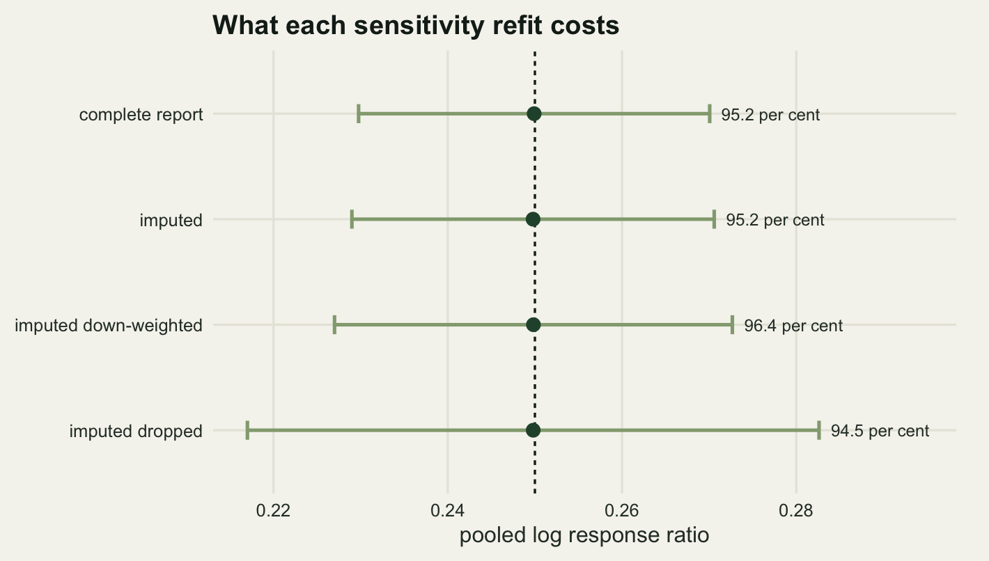
The imputed fraction is 60 per cent and the down-weighting multiplies an imputed study’s variance by 2. In the homogeneous corpus all four analyses put the pooled estimate on the truth to three decimal places, and all four cover it at close to the nominal rate. What separates them is width. The unobtainable complete-report analysis has a mean standard error of 0.01028; the full imputed analysis 0.01061, only 3.2 per cent wider, at a coverage of 95.2 per cent. Doubling the variances of the imputed studies takes the standard error to 0.01165, another 9.8 per cent, and pushes coverage to 96.4 per cent, which is conservative rather than better. Dropping the imputed studies takes the standard error to 0.01674, 57.8 per cent wider than keeping them, and returns a coverage of 94.5 per cent, which is no better than the analysis it was meant to check.
That is the clearest practical result in the post. Complete-case analysis is the most popular answer to a missing standard deviation and, on these numbers, the worst of the three: it makes the standard error 57.8 per cent larger and does not buy accuracy with it. Down-weighting costs 9.8 per cent and is a defensible hedge. Keeping the imputed studies at face value was, here, already fine.
The spread across the three analyst choices is 0.0103 on the log scale, which is 24.8 per cent of the width of the full analysis’s own confidence interval. The complete-case estimate sits 0.492 interval half-widths away from the full one on average. Those are the numbers a methods section would quote, and they look reassuring.
They should not be read as an interval. Across the replicates, the range between the three analyses contains the true effect only 30.2 per cent of the time, and at a between-study standard deviation of 0.15 it is 31.5 per cent. The reason is that the three analyses share most of their data, so they move together; their disagreement measures how much the analyst’s choice matters, not how much the estimate could be wrong. A sensitivity range of 24.8 per cent of the interval width is a statement about robustness to a decision, and reporting it alongside a confidence interval is right. Reporting it instead of one, or treating its endpoints as plausible values, is not. Nakagawa et al (2017) put the handling of missing statistics among the questions a reader of an ecological meta-analysis should be able to answer from the paper itself, and that is the standard the methods section has to meet.
One diagnostic does earn its place, and it needs no knowledge of the truth. The effective number of studies, one over the sum of squared normalised weights, is printable from the weights alone. In the display corpus it was 22.76 under correct standard errors and 5.49 under the misreading, so the units error announces itself loudly. Under quartile recovery it barely moves, which is the correct behaviour: the diagnostic fires for the error that matters and stays quiet for the one that does not.
What to take away
Reconstruction does not recover information that was never printed. It converts a missing number into an assumption with a name attached, and the useful output of this post is a set of sizes for what each assumption costs.
Recovering a standard deviation is far harder than recovering a mean. From a median and quartiles at an arm of 40, the mean comes back with a relative RMSE of 4.25 per cent and the standard deviation with 18.1 per cent. Among the recovery formulas, Hozo’s is the only one whose bias stays large at every arm size, running 7.42 per cent high at an arm of 40 and 18.98 per cent low just above its cut point at 70. Wan’s two estimators are close to unbiased and cross over in precision just above an arm of 80: use the range in small studies, the quartiles in large ones.
A standard error read as a standard deviation is a different order of problem. It multiplies a study’s inverse-variance weight by exactly its own sample size, so 7 such papers out of 30 took 96.4 per cent of the fixed-effect weight and cut the effective number of contributing studies from 22.76 to 5.49. Fixed-effect coverage fell from 93 per cent to 20.9 per cent in a homogeneous corpus. The random-effects model kept its coverage, at 91.6 per cent, and paid for it by reporting an I-squared of 85.2 per cent for a set of studies with no heterogeneity at all. If a synthesis finds surprisingly high heterogeneity in a literature you expected to be consistent, checking whether the error bars were all read the same way is cheaper than any moderator analysis.
Three things went against what I expected going in, and all three stay in. The correlation between a study’s weight and the error in its recovered standard deviation is real, negative and -0.59 over 300 studies, but it does not translate into a bias worth reporting: imputing every study rather than none shifted the pooled estimate by 6.84e-06 in the homogeneous corpus and -4.76e-07 at a between-study standard deviation of 0.2, both smaller than the Monte Carlo error on the shift itself and both against a true effect of 0.25. Coverage fell by about a point in the homogeneous case and by nothing detectable once heterogeneity was present. The protection comes from the same tau-squared that the rest of the meta-analysis thread treats as the problem: once it dominates the within-study variances, the weights flatten and stop caring what those variances were. An unbiased recovery error averages out over thirty studies; a systematic units error does not.
The sensitivity range is not the honest interval I assumed it would be either. Its width here was 24.8 per cent of the confidence interval, but it contained the true effect only 30.2 per cent of the time, because three refits of the same studies are not three independent estimates. Report it as a robustness statement and keep the confidence interval as the interval.
The third surprise is the one with a direct practical consequence. Dropping the imputed studies, which is the most common way of handling the problem and the one that feels most cautious, was the worst of the three refits: it widened the interval by 57.8 per cent and returned a coverage of 94.5 per cent against 95.2 per cent for simply keeping them. Caution that costs precision and buys no accuracy is not caution.
The limits of all of this are set by the simulation knowing the answer. Every error measured above is a distance from a value that was written down before the data were generated, and a real corpus has no such value. The recovery formulas were also given data drawn from the distribution they assume; on skewed biomass data, which is exactly why those studies printed a median in the first place, they would do worse than reported here, and by an amount nothing in the printed summary can reveal. So the measured biases are a best case rather than a bound on the damage, and the one durable conclusion is upstream of all of it: the fix for a missing standard deviation is a data availability statement, not a formula.
References
Hozo SP, Djulbegovic B, Hozo I 2005 BMC Medical Research Methodology 5:13 (10.1186/1471-2288-5-13)
Wan X, Wang W, Liu J, Tong T 2014 BMC Medical Research Methodology 14:135 (10.1186/1471-2288-14-135)
Luo D, Wan X, Liu J, Tong T 2018 Statistical Methods in Medical Research 27(6):1785-1805 (10.1177/0962280216669183)
Hedges LV, Gurevitch J, Curtis PS 1999 Ecology 80(4):1150-1156 (10.1890/0012-9658(1999)080[1150:TMAORR]2.0.CO;2)
Lajeunesse MJ 2015 Ecology 96(8):2056-2063 (10.1890/14-2402.1)
Wiebe N, Vandermeer B, Platt RW, Klassen TP, Moher D, Barrowman NJ 2006 Journal of Clinical Epidemiology 59(4):342-353 (10.1016/j.jclinepi.2005.08.017)
Weir CJ, Butcher I, Assi V, Lewis SC, Murray GD, Langhorne P, Brady MC 2018 BMC Medical Research Methodology 18:25 (10.1186/s12874-018-0483-0)
Nakagawa S, Noble DWA, Senior AM, Lagisz M 2017 BMC Biology 15:18 (10.1186/s12915-017-0357-7)