library(ggplot2)
library(patchwork)

te_paper  <- "#f5f4ee"
te_ink    <- "#16241d"
te_body   <- "#2c3a31"
te_forest <- "#275139"
te_rust   <- "#b5534e"
te_gold   <- "#c9b458"
te_line   <- "#dad9ca"

theme_datasheet <- function() {
  theme_minimal(base_size = 12) +
    theme(plot.background  = element_rect(fill = te_paper, colour = NA),
          panel.background = element_rect(fill = te_paper, colour = NA),
          panel.grid.major = element_line(colour = te_line, linewidth = 0.3),
          panel.grid.minor = element_blank(),
          text             = element_text(colour = te_body),
          plot.title       = element_text(colour = te_ink, face = "bold"),
          plot.subtitle    = element_text(colour = te_body),
          axis.text        = element_text(colour = te_body),
          strip.text       = element_text(colour = te_ink))
}Meta-analysis of little-replicated experiments
R
meta-analysis
response ratio
simulation
ecology tutorial
Three bottles per arm make the variance of a log response ratio an estimate too. Measuring in R what that does to coverage, tau-squared and Egger’s test.
A synthesis of nutrient limitation in lakes collects bottle bioassays: water from one lake, split into a control and a phosphorus addition, three bottles of each, chlorophyll after a few days. Each experiment becomes one log response ratio, the log of the treatment mean over the control mean, and each gets a sampling variance from the two arm means and standard deviations. Then the usual machinery runs: inverse-variance weights, a pooled effect with an interval, tau-squared and I-squared for the disagreement between lakes, Egger’s regression for small-study bias. Three bottles per arm is not a caricature. Bioassays are cheap to repeat across lakes and expensive to replicate within one, so the literature is full of them.
Every one of those statistics treats the within-study variance as known. The post on heterogeneity in meta-analysis says so in its limits: its interval for I-squared and its Q-profile interval for tau-squared “both assume the within-study variances are known”, an approximation that weakens with very small studies. With three bottles the variance is estimated from two degrees of freedom per arm, and the estimate is itself very noisy.
The closest earlier post is effect sizes from incomplete reports. Its section on a standard error read as a standard deviation shows a units error inventing between-study variance: the random-effects interval barely moves because tau-squared and I-squared absorb the damage. Its section on correlated weights then shows that honest, unbiased noise in a recovered standard deviation is almost free, with arms of eight to eighty plants. This post stays with honest reports and goes down to bioassay replication, where that noise is no longer free. At three bottles per arm, correctly reported variances do to a synthesis much of what the units error did, and the damage lands in the statistics a review reads as context dependence and publication bias.
None of this is new. Hedges, Gurevitch and Curtis 1999 derived the response ratio variance and warned about small samples, Lajeunesse 2015 gave a second-order correction for the ratio and its variance, Doncaster and Spake 2018 measured the bias from little-replicated studies and proposed replacing each study’s variance component by its mean across studies, and Pustejovsky and Rodgers 2019 showed Egger’s test misfiring on standardised mean differences. The post is a demonstration of those results in a bioassay setting, with every number computed below. It ends with the standardised mean difference version of the Egger problem, which the posts on checking for publication bias and selection models mention in their limits without measuring.
Three bottles give a variance that is an estimate
Each simulated experiment draws chlorophyll in every bottle from a lognormal distribution with a given coefficient of variation, the control arm with mean one and the treatment arm with mean equal to the exponential of the true log response ratio, 0.3. With between-lake heterogeneity the treatment mean of each lake is drawn around that value. The function returns, for many syntheses at once, the log response ratio of every study and the squared sample coefficient of variation of each arm, which is all the variance formula needs.
lnrr_true <- 0.3                    # true log response ratio
k_grid    <- c(5, 20, 80)           # studies per synthesis
n_grid    <- c(3, 6, 10)            # bottles per arm
cv_grid   <- c(0.3, 0.6, 0.8)       # coefficient of variation of a bottle
n_meta    <- 1000                   # simulated syntheses per cell, fixed in advance
z_crit    <- qnorm(0.975)

bottles <- function(R, k, n, cv, cv_t = cv, tau = 0, n_vec = rep(n, k)) {
  # n_vec: one bottle number per study, or an R by k matrix (one row per synthesis)
  n_mat <- if (is.matrix(n_vec)) n_vec else matrix(n_vec, R, k, byrow = TRUE)
  n_max <- max(n_mat)
  sdl_c <- sqrt(log(1 + cv^2)); sdl_t <- sqrt(log(1 + cv_t^2))
  theta <- matrix(lnrr_true + rnorm(R * k, 0, tau), R, k)
  xc <- array(rlnorm(R * k * n_max, -sdl_c^2 / 2, sdl_c), c(R, k, n_max))
  xt <- array(rlnorm(R * k * n_max, -sdl_t^2 / 2, sdl_t), c(R, k, n_max)) *
        as.vector(exp(theta))
  keep <- array(outer(as.vector(n_mat), seq_len(n_max), ">="), c(R, k, n_max))
  arm_sum <- function(x) apply(x * keep, c(1, 2), sum)
  mc <- arm_sum(xc) / n_mat; mt <- arm_sum(xt) / n_mat
  sc2 <- (arm_sum(xc^2) - n_mat * mc^2) / (n_mat - 1)
  st2 <- (arm_sum(xt^2) - n_mat * mt^2) / (n_mat - 1)
  list(y = log(mt / mc), cvc2 = sc2 / mc^2, cvt2 = st2 / mt^2, n = n_mat)
}
The sampling variance of the log response ratio from Hedges, Gurevitch and Curtis 1999 is the squared coefficient of variation of each arm divided by its sample size, summed over the two arms. With the true coefficients of variation plugged in it is a constant for a given design; with the sample values plugged in, as every synthesis does, it is a random quantity. Draw many single experiments and compare the two.
set.seed(1150)
n_single <- 20000
single <- do.call(rbind, lapply(n_grid, function(nn) {
  b <- bottles(n_single, 1, nn, 0.6)
  v_hat <- (b$cvc2 + b$cvt2) / nn
  data.frame(n = nn, ratio = as.vector(v_hat) / (2 * 0.6^2 / nn),
             y = as.vector(b$y))
}))
single$n_lab <- factor(sprintf("%d bottles per arm", single$n),
                       levels = sprintf("%d bottles per arm", n_grid))
rat_med  <- tapply(single$ratio, single$n, median)
rat_half <- tapply(single$ratio < 0.5, single$n, mean)
rat_q    <- tapply(single$ratio, single$n, quantile, probs = 0.95)
rat_q05  <- tapply(single$ratio, single$n, quantile, probs = 0.05)
var_y    <- tapply(single$y, single$n, var)
With three bottles per arm and a bottle coefficient of variation of 0.6, the median estimated variance is 0.63 of the value the formula gives with the true coefficient of variation, 38 per cent of experiments report less than half of it, and the upper 5 per cent report more than 1.7 times it. With ten bottles the median is 0.81 and the share below half is 11 per cent. The inverse of that variance is the study’s weight, so at three bottles an experiment at the lower 5 per cent point of the variance distribution is weighted 11 times more than an identical experiment at the upper 5 per cent point; at ten bottles the factor is 4.
ggplot(single, aes(ratio)) +
  geom_histogram(bins = 60, fill = te_forest, colour = te_paper, linewidth = 0.15) +
  geom_vline(xintercept = 1, colour = te_rust, linetype = "dashed", linewidth = 0.8) +
  scale_x_log10(breaks = c(0.1, 0.3, 1, 3, 10), labels = c("0.1", "0.3", "1", "3", "10")) +
  facet_wrap(~ n_lab, ncol = 1) +
  labs(x = "estimated variance / variance at the true CV (log scale)", y = "experiments",
       title = "The variance of a three-bottle ratio is a guess",
       subtitle = "dashed line: the variance with the true coefficient of variation") +
  theme_datasheet()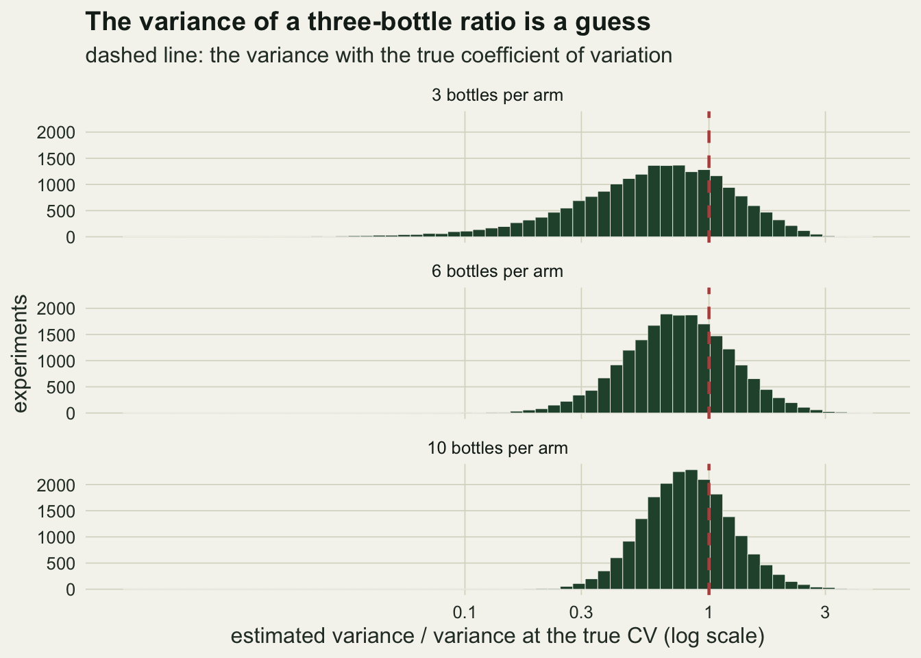
Fixed-effect coverage falls as studies are added
Four ways of pooling the same simulated studies, each with a nominal 95 per cent interval. Inverse-variance weights with each study’s own estimated variance are the default. The Lajeunesse 2015 version adds half the difference of the two squared-CV terms to the ratio and a second-order term to its variance. The pooled-CV version follows Doncaster and Spake 2018 in replacing each arm’s squared coefficient of variation by its mean across the studies in the synthesis, so that only sample size moves the weights. The last is the unweighted mean of the ratios with a t interval on k minus one degrees of freedom.
pool_fe <- function(y, v) {
  w <- 1 / v; sw <- rowSums(w)
  list(mu = rowSums(w * y) / sw, se = sqrt(1 / sw), top = apply(w, 1, max) / sw)
}
covers <- function(mu, se, crit) abs(mu - lnrr_true) <= crit * se
fixed_cell <- function(b) {
  k <- ncol(b$y)
  v_own  <- (b$cvc2 + b$cvt2) / b$n
  y_laj  <- b$y + 0.5 * (b$cvt2 - b$cvc2) / b$n
  v_laj  <- v_own + 0.5 * (b$cvt2^2 + b$cvc2^2) / b$n^2
  v_pool <- (rowMeans(b$cvc2) + rowMeans(b$cvt2)) / b$n
  own <- pool_fe(b$y, v_own); laj <- pool_fe(y_laj, v_laj); pld <- pool_fe(b$y, v_pool)
  unw_mu <- rowMeans(b$y); unw_se <- sqrt(apply(b$y, 1, var) / k)
  c(own = mean(covers(own$mu, own$se, z_crit)),
    lajeunesse = mean(covers(laj$mu, laj$se, z_crit)),
    pooled_cv = mean(covers(pld$mu, pld$se, z_crit)),
    unweighted = mean(covers(unw_mu, unw_se, qt(0.975, k - 1))),
    bias_own = mean(own$mu) - lnrr_true, bias_laj = mean(laj$mu) - lnrr_true,
    bias_unw = mean(unw_mu) - lnrr_true, bias_unw_laj = mean(rowMeans(y_laj)) - lnrr_true,
    sd_ratio = sd(own$mu) / mean(own$se), top_share = median(own$top))
}
fx_grid <- expand.grid(k = k_grid, n = n_grid, cv = cv_grid)
set.seed(2056)
fx <- cbind(fx_grid, t(vapply(seq_len(nrow(fx_grid)), function(i)
  fixed_cell(bottles(n_meta, fx_grid$k[i], fx_grid$n[i], fx_grid$cv[i])), numeric(10))))
fx_at <- function(k, n, cv, col) fx[fx$k == k & fx$n == n & fx$cv == cv, col]
mcse_cov <- sqrt(0.95 * 0.05 / n_meta)
unw_rng <- range(fx$unweighted)
pool_n3 <- range(fx$pooled_cv[fx$n == 3]); pool_all <- range(fx$pooled_cv)
laj_gap <- max(abs(fx$lajeunesse - fx$own)); bias_max <- max(abs(fx$bias_own))
own_n10 <- range(fx$own[fx$n == 10]); own_n6 <- range(fx$own[fx$n == 6])
drop_n6 <- sapply(cv_grid, function(cv) fx_at(5, 6, cv, "own") - fx_at(80, 6, cv, "own"))
drop_n10 <- sapply(cv_grid, function(cv) fx_at(5, 10, cv, "own") - fx_at(80, 10, cv, "own"))
At three bottles per arm and a coefficient of variation of 0.3, own-variance weights cover the true ratio in 0.768 of syntheses of five studies, 0.678 of syntheses of twenty and 0.634 of syntheses of eighty, with a Monte Carlo standard error of 0.007 near 0.95. The coverage gets worse as the evidence grows. At a coefficient of variation of 0.8 the same three numbers are 0.748, 0.671 and 0.623. With six bottles the coverage sits between 0.839 and 0.889 across the grid and still falls a little from five to eighty studies in every panel, by 0.010 to 0.027. With ten bottles it sits between 0.879 and 0.913, and the change from five to eighty studies runs from 0.004 to 0.009. Both are short of nominal.
The pooled estimate is not biased: the largest mean error in the grid is 0.007 on a true value of 0.3. The failure is entirely in the interval. At three bottles and eighty studies the actual spread of the pooled estimate is 2.39 times its mean reported standard error, against 1.59 times at five studies. The reason it grows with k is in the weights. In a synthesis of eighty three-bottle studies the heaviest study carries a median 0.090 of the total weight, 7.2 times its fair share of one eightieth; with ten bottles the same figure is 2.4 times. The weights have such a long tail at two degrees of freedom per arm that adding studies keeps finding a new lucky one, and the reported standard error shrinks faster than the estimate settles.
fx$n_lab <- factor(sprintf("%d bottles", fx$n), levels = sprintf("%d bottles", n_grid))
fx$cv_lab <- factor(sprintf("CV %.1f", fx$cv), levels = sprintf("CV %.1f", cv_grid))
ggplot(fx, aes(k, own, colour = n_lab)) +
  geom_hline(yintercept = 0.95, colour = te_body, linetype = "dashed", linewidth = 0.5) +
  geom_line(linewidth = 0.9) + geom_point(size = 2.2) +
  scale_x_log10(breaks = k_grid) +
  scale_colour_manual(values = c(te_rust, te_gold, te_forest), name = NULL) +
  scale_y_continuous(limits = c(0.5, 1)) +
  facet_wrap(~ cv_lab) +
  labs(x = "studies in the synthesis (log scale)", y = "coverage",
       title = "More three-bottle studies, worse intervals",
       subtitle = "own-variance weights; dashed line: nominal 0.95") +
  theme_datasheet() + theme(legend.position = "bottom")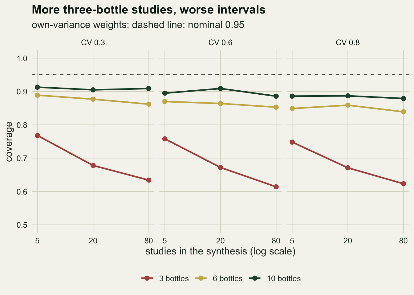
The Lajeunesse correction does not help here, and it was never meant to: its largest difference from the uncorrected coverage anywhere in the grid is 0.007. It corrects a bias in the ratio, and with equal coefficients of variation in the two arms there is almost none to correct. The weights, not the ratio, are the problem, and the two ways of pooling that stop the weights from reading the noise both repair most of it. At equal replication the pooled-CV weights are all equal, so the two give the same pooled ratio; they differ only in the standard error, the pooled-CV one computed from the averaged coefficients of variation, which are biased low (see the random-effects section), and the t interval from the observed spread of the ratios. Pooled-CV weights cover between 0.901 and 0.944 at three bottles, and the unweighted mean with a t interval covers between 0.940 and 0.962 across the whole grid.
set.seed(2057)
uneq <- t(vapply(k_grid, function(k)
  fixed_cell(bottles(n_meta, k, 3, 0.6, cv_t = 0.72)), numeric(10)))
bias_delta <- -(0.72^2 - 0.6^2) / (2 * 3)
one_uneq <- bottles(n_single, 1, 3, 0.6, cv_t = 0.72)
cor_t <- cor(as.vector(one_uneq$y), as.vector(one_uneq$cvt2))
cor_c <- cor(as.vector(one_uneq$y), as.vector(one_uneq$cvc2))
Unequal spread is the case the correction was built for. Give the treatment bottles a coefficient of variation 1.2 times the control’s, 0.72 against 0.6, and the log of a three-bottle mean is pulled down more in the treatment arm; the second-order approximation to that pull is -0.026. At eighty studies the unweighted mean of the uncorrected ratios is off by -0.021 and the unweighted mean of the corrected ratios by -0.008. The inverse-variance estimate is off by more, -0.038 uncorrected and -0.034 corrected, because the noisy weights add a bias of their own that the correction does not touch: with skewed bottles, an arm whose mean came out high tends to report a high coefficient of variation too. In single three-bottle experiments of this kind the ratio correlates 0.25 with the treatment squared coefficient of variation and -0.16 with the control one, so the weight and the ratio are not independent, and with unequal arms the two correlations no longer cancel. Coverage at eighty studies is 0.539 uncorrected, 0.542 corrected and 0.922 for the unweighted t interval. Applied to an unweighted mean, then, the correction removes most of the pull; applied inside an inverse-variance fit it cannot reach the part the weights add.
est_lev <- c("own variance", "Lajeunesse", "pooled CV", "unweighted t")
fx3 <- fx[fx$n == 3, ]
est <- data.frame(k = rep(fx3$k, 4), cv_lab = rep(fx3$cv_lab, 4),
                  method = factor(rep(est_lev, each = nrow(fx3)), levels = est_lev),
                  coverage = c(fx3$own, fx3$lajeunesse, fx3$pooled_cv, fx3$unweighted))
ggplot(est, aes(k, coverage, colour = method, linetype = method)) +
  geom_hline(yintercept = 0.95, colour = te_body, linetype = "dashed", linewidth = 0.5) +
  geom_line(linewidth = 0.9) + geom_point(size = 2) +
  scale_x_log10(breaks = k_grid) +
  scale_colour_manual(values = c(te_rust, te_gold, te_forest, te_ink), name = NULL) +
  scale_linetype_manual(values = c("solid", "dotted", "solid", "solid"), name = NULL) +
  scale_y_continuous(limits = c(0.5, 1)) +
  facet_wrap(~ cv_lab) +
  labs(x = "studies in the synthesis (log scale)", y = "coverage",
       title = "Weights that ignore the noise hold up",
       subtitle = "three bottles per arm; dashed line: nominal 0.95") +
  theme_datasheet() + theme(legend.position = "bottom")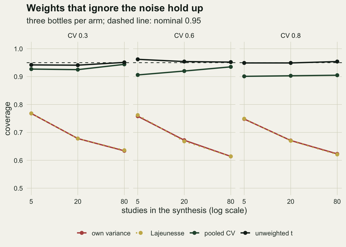
Random effects buy back coverage with tau-squared
A synthesis across lakes would normally use a random-effects model, so the more relevant question is what the random-effects model does with the same noisy variances. Tau-squared is estimated two ways: DerSimonian-Laird from Cochran’s Q, and REML by Fisher scoring, iterated from the DerSimonian-Laird value and truncated at zero, both written out so the only thing that changes between them is the estimator. The interval is the usual normal one, and a Knapp-Hartung interval on k minus one degrees of freedom is added as the small-k alternative. Here the coefficient of variation is fixed at 0.6 and the true between-lake standard deviation is either zero or 0.2, a tau-squared of 0.04.
tau_grid <- c(0, 0.2)
tau2_dl <- function(y, v) {
  w <- 1 / v; sw <- rowSums(w); mu <- rowSums(w * y) / sw
  Q <- rowSums(w * (y - mu)^2); k <- ncol(y)
  list(t2 = pmax(0, (Q - (k - 1)) / (sw - rowSums(w^2) / sw)), Q = Q)
}
tau2_reml <- function(y, v, start, n_iter = 100) {
  t2 <- start
  for (i in seq_len(n_iter)) {
    w <- 1 / (v + t2); sw <- rowSums(w); mu <- rowSums(w * y) / sw
    t2 <- pmax(0, rowSums(w^2 * ((y - mu)^2 - v)) / rowSums(w^2) + 1 / sw)
  }
  t2
}
random_cell <- function(b) {
  k <- ncol(b$y); out <- NULL
  v_list <- list(own = (b$cvc2 + b$cvt2) / b$n,
                 pooled = (rowMeans(b$cvc2) + rowMeans(b$cvt2)) / b$n)
  for (nm in names(v_list)) {
    v <- v_list[[nm]]; d <- tau2_dl(b$y, v); r2 <- tau2_reml(b$y, v, d$t2)
    w <- 1 / (v + d$t2); sw <- rowSums(w); mu <- rowSums(w * b$y) / sw
    se_hk <- sqrt(rowSums(w * (b$y - mu)^2) / ((k - 1) * sw))
    wr <- 1 / (v + r2); mur <- rowSums(wr * b$y) / rowSums(wr)
    out <- c(out, setNames(c(mean(d$t2), mean(r2), mean(pmax(0, (d$Q - (k - 1)) / d$Q)),
      mean(covers(mu, sqrt(1 / sw), z_crit)), mean(covers(mu, se_hk, qt(0.975, k - 1))),
      mean(covers(mur, sqrt(1 / rowSums(wr)), z_crit))),
      paste(nm, c("dl", "reml", "i2", "cov_dl", "cov_hk", "cov_reml"), sep = "_")))
  }
  out
}
re_grid <- expand.grid(k = k_grid, n = n_grid, tau = tau_grid)
set.seed(634)
re <- cbind(re_grid, t(vapply(seq_len(nrow(re_grid)), function(i)
  random_cell(bottles(n_meta, re_grid$k[i], re_grid$n[i], 0.6, tau = re_grid$tau[i])),
  numeric(12))))
re_at <- function(k, n, tau, col) re[re$k == k & re$n == n & re$tau == tau, col]
v_gap3 <- var_y["3"] - mean(single$ratio[single$n == 3]) * 2 * 0.6^2 / 3
With a true tau-squared of 0.04 and three bottles per arm, the DerSimonian-Laird estimate with own variances averages 0.148, 0.148 and 0.148 at five, twenty and eighty studies, so the inflation does not shrink with more studies; with ten bottles it averages 0.054 at eighty. The random-effects interval covers 0.881, 0.920 and 0.937 at the three study counts. So the random-effects interval climbs back towards nominal as studies are added, where the fixed-effect interval fell away, and it does it the way the units error did in the incomplete-reports post: the scatter the noisy weights cannot explain is booked as between-lake variance, and every study’s weight is flattened by it.
The inflation does not need any heterogeneity. In homogeneous syntheses of eighty three-bottle studies, where every lake has exactly the same response, tau-squared averages 0.109 and I-squared averages 49 per cent. With ten bottles the homogeneous values are 0.014 and 18 per cent.
Pooled-CV variances remove part of it, not all. At three bottles, eighty studies and no heterogeneity their tau-squared still averages 0.046. That remainder has a different source, and the single-experiment draws above price it. The actual variance of a three-bottle log response ratio at a coefficient of variation of 0.6 is 0.221, and the variance formula with sample coefficients of variation averages 0.176, mostly because a sample coefficient of variation from three skewed values is biased low (the formula with the true value, 0.240, is itself slightly above the actual variance, so the gap is the net of the two). The gap is 0.045, which is what a correctly weighted synthesis must then call heterogeneity. Averaging the coefficients of variation across studies removes their noise but not their bias.
tau_long <- data.frame(
  k = rep(re$k, 2), n_lab = factor(rep(sprintf("%d bottles", re$n), 2),
                                   levels = sprintf("%d bottles", n_grid)),
  tau_lab = factor(rep(ifelse(re$tau == 0, "true tau-squared 0", "true tau-squared 0.04"), 2)),
  truth = rep(re$tau^2, 2),
  variance = factor(rep(c("own variance", "pooled CV"), each = nrow(re)),
                    levels = c("own variance", "pooled CV")),
  tau2 = c(re$own_dl, re$pooled_dl))
ggplot(tau_long, aes(k, tau2, colour = n_lab, linetype = variance)) +
  geom_hline(aes(yintercept = truth), colour = te_body, linetype = "dashed", linewidth = 0.5) +
  geom_line(linewidth = 0.9) + geom_point(size = 2) +
  scale_x_log10(breaks = k_grid) +
  scale_colour_manual(values = c(te_rust, te_gold, te_forest), name = NULL) +
  scale_linetype_manual(values = c("solid", "dotted"), name = NULL) +
  scale_y_continuous(limits = c(0, NA)) +
  facet_wrap(~ tau_lab) +
  guides(colour = guide_legend(nrow = 1), linetype = guide_legend(nrow = 1)) +
  labs(x = "studies in the synthesis (log scale)", y = "mean estimated tau-squared",
       title = "Heterogeneity made of bottle noise",
       subtitle = "dashed line: the true tau-squared") +
  theme_datasheet() + theme(legend.position = "bottom", legend.box = "vertical")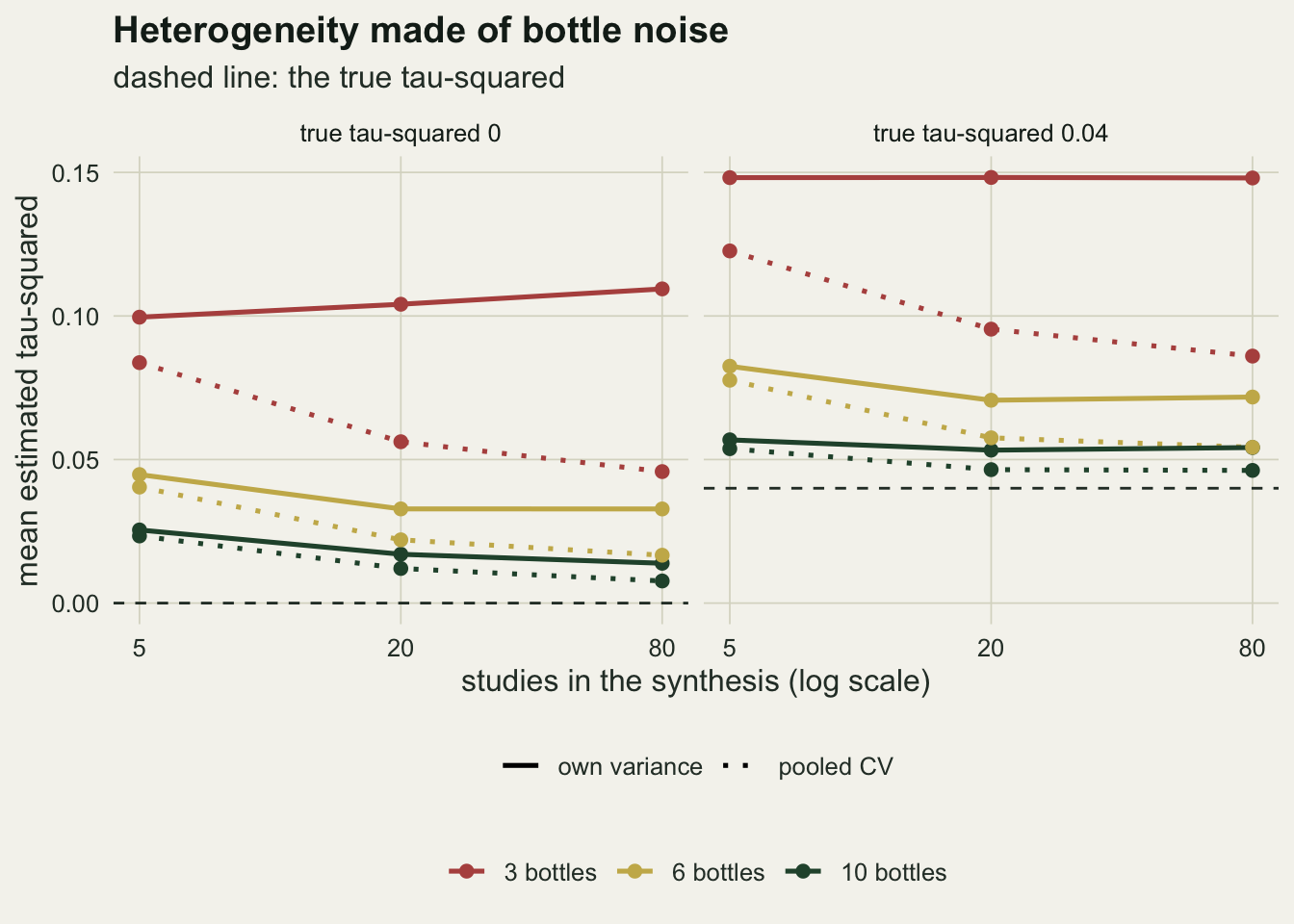
REML does not change the picture. At three bottles and a true tau-squared of 0.04 it averages 0.141, 0.137 and 0.137 at the three study counts, a little below DerSimonian-Laird and still more than three times the truth; its interval covers 0.890 at five studies. At five studies the choice that moves coverage is the interval, not the tau-squared estimator. At five studies and three bottles the Knapp-Hartung interval with own variances covers 0.919 and with pooled-CV variances 0.945 (at equal bottle numbers this is exactly the unweighted t interval), against 0.881 for the normal interval with own variances.
Egger’s test accuses an honest literature
Egger’s regression divides each effect by its standard error and regresses that on precision, one over the standard error; an intercept away from zero is read as small-study bias. The simulated syntheses below have no selection of any kind, so every rejection at the 5 per cent level is a false alarm. Twenty studies per synthesis, no heterogeneity, and either all studies with three bottles per arm, or bottle numbers between three and ten drawn afresh for every study in every synthesis, so that the rate averages over many mixed designs rather than describing one.
egger_t <- function(y, se) {
  z <- y / se; x <- 1 / se; k <- ncol(y)
  xm <- rowMeans(x); zm <- rowMeans(z); sxx <- rowSums((x - xm)^2)
  b1 <- rowSums((x - xm) * (z - zm)) / sxx; b0 <- zm - b1 * xm
  s2 <- rowSums((z - b0 - b1 * x)^2) / (k - 2)
  b0 / sqrt(s2 * (1 / k + xm^2 / sxx))
}
n_egger <- 4000; k_egger <- 20; crit_e <- qt(0.975, k_egger - 2)
egger_cases <- list("3 bottles" = c(3, 3), "3 to 10 bottles" = c(3, 10),
                    "6 bottles" = c(6, 6), "10 bottles" = c(10, 10))
set.seed(629)
eg <- do.call(rbind, lapply(c(0.3, 0.8), function(cv) do.call(rbind,
  lapply(names(egger_cases), function(nm) {
    rr <- egger_cases[[nm]]
    n_vec <- if (rr[1] == rr[2]) rep(rr[1], k_egger) else
      matrix(sample(rr[1]:rr[2], n_egger * k_egger, TRUE), n_egger, k_egger)
    b <- bottles(n_egger, k_egger, NA, cv, n_vec = n_vec)
    se_own <- sqrt((b$cvc2 + b$cvt2) / b$n)
    y_noise <- matrix(rnorm(n_egger * k_egger, lnrr_true, 0.3), n_egger, k_egger)
    se_pool <- sqrt((rowMeans(b$cvc2) + rowMeans(b$cvt2)) / b$n)
    data.frame(cv = cv, design = nm,
               own = mean(abs(egger_t(b$y, se_own)) > crit_e),
               pooled = if (rr[1] == rr[2]) NA else mean(abs(egger_t(b$y, se_pool)) > crit_e),
               noise = mean(abs(egger_t(y_noise, se_own)) > crit_e))
  }))))
eg$design <- factor(eg$design, levels = names(egger_cases))
eg_at <- function(cv, nm, col) eg[eg$cv == cv & eg$design == nm, col]
mcse_e <- sqrt(0.05 * 0.95 / n_egger)
With every study at three bottles, Egger’s test flags small-study bias in 0.136 of honest syntheses at a coefficient of variation of 0.3 and 0.133 at 0.8, against a nominal 0.05 and a Monte Carlo standard error of 0.003. A literature of mixed replication, three to ten bottles, gives 0.076 and 0.069; all six bottles gives 0.084 and 0.079, and all ten bottles gives 0.061 and 0.054.
The mechanism is not a correlation between the ratio and its standard error. The second column of the calculation keeps each study’s noisy standard error and replaces its ratio with a normal draw, mean 0.3 and standard deviation 0.3, that has nothing to do with the bottles. Egger’s test still rejects in 0.149 of those syntheses with three bottles, and in 0.066 with ten. The regression assumes the standardised effect has the same variance at every precision. With an estimated standard error it does not: a study whose variance came out too small has a large precision and a standardised effect scattered far too widely, so the few most precise-looking studies have both the most pull on the fitted line and the largest residuals, and the ordinary t statistic for the intercept is too large. Pooled-CV standard errors vary only with the bottle numbers. In the mixed three-to-ten literature they bring the rate to 0.051 and 0.048 at the two coefficients of variation; with equal bottle numbers they leave Egger’s test nothing to regress on, since every study has the same precision.
The same false alarm with standardised mean differences
Pustejovsky and Rodgers 2019 describe a different mechanism with the same symptom for Hedges’ g. Its usual variance, the sum of the inverse arm sizes plus the squared effect divided by twice the total sample size, contains the effect itself, so a larger g carries a larger standard error in every study, and funnel asymmetry appears as soon as the true effect is not zero. Their modified test replaces the standard error by a quantity that depends only on the sample sizes, the square root of the sum of the inverse arm sizes. In the version used here that quantity replaces the standard error both as the predictor and in the standardisation.
The simulation draws the difference in arm means and the pooled variance from their exact normal and chi-squared distributions, equal arms drawn once per study between 5 and 20 or between 20 and 60, a between-study standard deviation of 0.1, and no selection.
sim_smd <- function(R, k, d, tau, n_lo, n_hi) {
  n_arm <- matrix(sample(n_lo:n_hi, R * k, replace = TRUE), R, k)
  theta <- d + matrix(rnorm(R * k, 0, tau), R, k)
  mean_diff <- theta + rnorm(R * k, 0, sqrt(2 / n_arm))
  s_pool2 <- rchisq(R * k, 2 * n_arm - 2) / (2 * n_arm - 2)
  g <- (1 - 3 / (4 * 2 * n_arm - 9)) * mean_diff / sqrt(s_pool2)
  se_std <- sqrt(2 / n_arm + g^2 / (4 * n_arm))
  se_n   <- sqrt(2 / n_arm)
  crit <- qt(0.975, k - 2)
  c(standard = mean(abs(egger_t(g, se_std)) > crit),
    n_only = mean(abs(egger_t(g, se_n)) > crit))
}
d_grid <- c(0, 0.4, 0.8, 1.2)
smd_grid <- expand.grid(d = d_grid, k = c(20, 40), arms = c("5 to 20", "20 to 60"),
                        stringsAsFactors = FALSE)
set.seed(57)
smd <- cbind(smd_grid, t(vapply(seq_len(nrow(smd_grid)), function(i) {
  lo_hi <- if (smd_grid$arms[i] == "5 to 20") c(5, 20) else c(20, 60)
  sim_smd(n_egger, smd_grid$k[i], smd_grid$d[i], 0.1, lo_hi[1], lo_hi[2])
}, numeric(2))))
smd_at <- function(d, k, arms, col) smd[smd$d == d & smd$k == k & smd$arms == arms, col]
nonly_rng <- range(smd$n_only)
With twenty studies of 5 to 20 animals per arm and no true effect, the standard test rejects in 0.051 of syntheses and the sample-size version in 0.045. At a true effect of 0.8 the standard test rejects in 0.118 and at 1.2 in 0.175, while the sample-size version gives 0.045 and 0.049. Larger arms of 20 to 60 soften the standard test to 0.127 at an effect of 1.2, and doubling the synthesis to forty studies of 5 to 20 raises it to 0.335. Across every cell the sample-size version stays between 0.041 and 0.054. A standard Egger test on g gains power to detect a bias that does not exist as the literature grows, and it misfires more the larger the true effect.
eg$cv_lab <- factor(sprintf("CV %.1f", eg$cv))
p_lnrr <- ggplot(eg, aes(design, own, fill = cv_lab)) +
  geom_col(position = position_dodge(width = 0.75), width = 0.65,
           colour = te_paper, linewidth = 0.3) +
  geom_hline(yintercept = 0.05, colour = te_body, linetype = "dashed", linewidth = 0.5) +
  scale_fill_manual(values = c(te_gold, te_rust), name = NULL) +
  scale_y_continuous(limits = c(0, NA)) +
  labs(x = NULL, y = "rejection rate, no bias present",
       title = "Response ratios", subtitle = "own standard errors") +
  theme_datasheet() +
  theme(legend.position = "bottom", axis.text.x = element_text(angle = 25, hjust = 1))

smd_long <- data.frame(
  d = rep(smd$d, 2),
  setting = factor(rep(sprintf("k %d, arms %s", smd$k, smd$arms), 2),
                   levels = c("k 20, arms 5 to 20", "k 20, arms 20 to 60", "k 40, arms 5 to 20",
                              "k 40, arms 20 to 60")),
  version = factor(rep(c("standard SE", "sample-size SE"), each = nrow(smd)),
                   levels = c("standard SE", "sample-size SE")),
  rate = c(smd$standard, smd$n_only))
p_smd <- ggplot(smd_long, aes(d, rate, colour = setting, linetype = version)) +
  geom_hline(yintercept = 0.05, colour = te_body, linetype = "dotted", linewidth = 0.4) +
  geom_line(linewidth = 0.9) + geom_point(aes(shape = version), size = 2, fill = te_paper) +
  scale_colour_manual(values = c(te_rust, te_gold, te_forest, te_ink), name = NULL) +
  scale_linetype_manual(values = c("solid", "dashed"), name = NULL) +
  scale_shape_manual(values = c(16, 21), name = NULL) +
  scale_y_continuous(limits = c(0, NA)) +
  guides(colour = guide_legend(ncol = 1), linetype = guide_legend(ncol = 1),
         shape = guide_legend(ncol = 1)) +
  labs(x = "true standardised mean difference", y = NULL,
       title = "Hedges' g", subtitle = "no selection, tau 0.1; dotted line: 0.05") +
  theme_datasheet() + theme(legend.position = "bottom", legend.box = "horizontal")

p_lnrr + p_smd + plot_layout(widths = c(1, 1.3)) + plot_annotation(theme = theme_datasheet())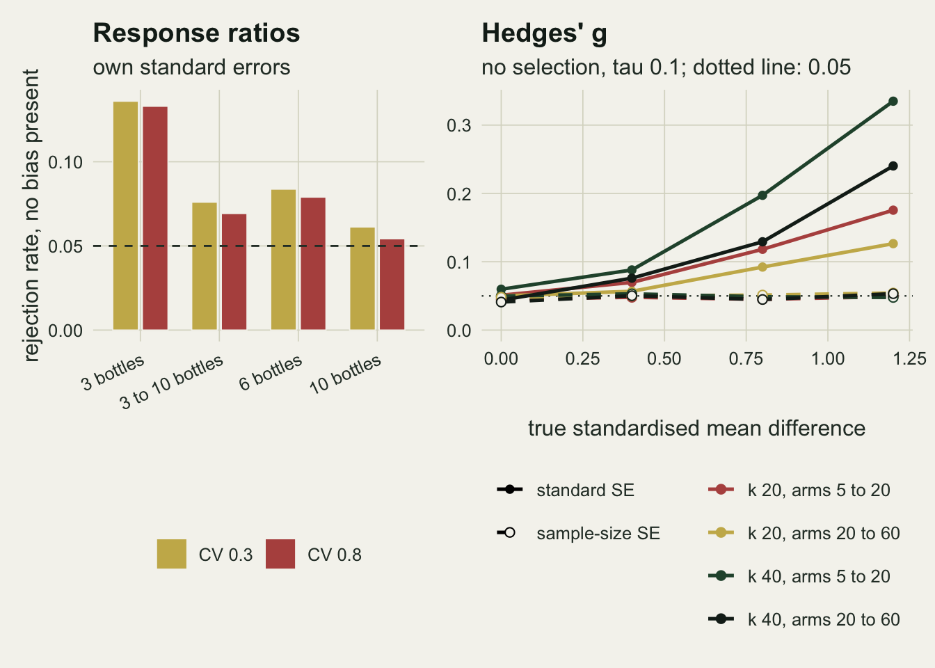
What to report
Report the replication of the included studies, as a distribution, before any pooled number. A reader who knows that most studies had three bottles per arm knows that the tau-squared, the I-squared and any funnel test that follows are partly statements about bottle noise.
Do not use each study’s own sampling variance as its weight at bioassay replication. In these simulations own-variance weights fell short of nominal even at ten bottles per arm, while the unweighted mean with a t interval held nominal coverage everywhere in the equal-spread grid, and pooled-CV weights stayed within five points of nominal at three bottles. At equal replication the two share a point estimate, and the unweighted mean with a t interval (identical to a Knapp-Hartung interval on pooled-CV weights) is the primary analysis; pooled-CV weights with a normal interval are the ones that undercover, by up to that margin. The default inverse-variance fit is the one that failed, and at three bottles per arm the failure grew with the size of the review.
Report tau-squared and I-squared from a pooled-CV fit next to the default fit. The difference between them is an estimate of how much of the reported heterogeneity is noise in the weights. What is left after pooling still contains the downward bias of small-sample coefficients of variation, so a residual tau-squared of a few hundredths at three bottles is not evidence of context dependence either.
Use the Lajeunesse correction when the two arms are likely to differ in spread, which a nutrient addition that produces blooms in some bottles and not others can do, and pair it with weights that do not read the noise: at three bottles it removed most of the bias of an unweighted mean and little of an inverse-variance one.
Do not run Egger’s test with study-level estimated standard errors on three-bottle log response ratios, and do not run the standard version on Hedges’ g when effects may be moderate or large. For g use a sample-size-based precision, as Pustejovsky and Rodgers 2019 recommend, and say which version was used.
Honest limits
Bottles here are independent lognormal draws, and arms within a study are independent. Real bioassay bottles share a carboy of lake water, an incubator shelf and a sampling day, so their errors need not be independent, within an arm or between the two arms. Correlated arms change the variance formula itself, which nothing here models.
The coefficient of variation was the same in every study of a synthesis, apart from the one unequal-arm case. That is the condition under which pooled-CV weights are exactly right about the spread and wrong only about its noise. Where lakes genuinely differ in bottle variability, averaging the coefficients of variation discards real information, and the pooled-CV numbers above may be optimistic.
The unweighted mean ignores sample size by construction. It did well here because the designs within a cell were identical or nearly so. A synthesis mixing three-bottle studies with mesocosm experiments of twenty replicates would pay for equal weights in width, and the comparison would have to be rerun on that mix.
Every rate is conditional on no selection. The Egger results say how often the test fires on an honest literature; they say nothing about its power against a filtered one, and a sample-size-based version may lose some of that power. The standardised mean difference section also uses one between-study standard deviation of 0.1 and equal arm sizes within studies.
Whether three bottles and coefficients of variation of 0.3 to 0.8 describe any particular synthesis, such as the freshwater bioassays compiled for nutrient limitation reviews, was not checked against those data. Replicate bottles filled from one well-mixed carboy may vary less than the middle of the grid; the fixed-effect failure above is already present at a coefficient of variation of 0.3, but the tau-squared section used 0.6 only. The grid was fixed before any rate was computed, and the numbers belong to it.
References
Hedges LV, Gurevitch J, Curtis PS 1999 Ecology 80(4):1150-1156 (10.1890/0012-9658(1999)080[1150:TMAORR]2.0.CO;2)
Lajeunesse MJ 2015 Ecology 96(8):2056-2063 (10.1890/14-2402.1)
Doncaster CP, Spake R 2018 Methods in Ecology and Evolution 9(3):634-644 (10.1111/2041-210X.12927)
Pustejovsky JE, Rodgers MA 2019 Research Synthesis Methods 10(1):57-71 (10.1002/jrsm.1332)
Egger M, Davey Smith G, Schneider M, Minder C 1997 BMJ 315(7109):629-634 (10.1136/bmj.315.7109.629)