library(ggplot2)
library(patchwork)
library(nlme)

te_paper  <- "#f5f4ee"
te_ink    <- "#16241d"
te_body   <- "#2c3a31"
te_forest <- "#275139"
te_rust   <- "#b5534e"
te_gold   <- "#c9b458"
te_line   <- "#dad9ca"

theme_datasheet <- function() {
  theme_minimal(base_size = 12) +
    theme(plot.background  = element_rect(fill = te_paper, colour = NA),
          panel.background = element_rect(fill = te_paper, colour = NA),
          panel.grid.major = element_line(colour = te_line, linewidth = 0.3),
          panel.grid.minor = element_blank(),
          text             = element_text(colour = te_body),
          plot.title       = element_text(colour = te_ink, face = "bold"),
          plot.subtitle    = element_text(colour = te_body),
          axis.text        = element_text(colour = te_body))
}Fitting a senescence model to individual records
R
nlme
mixed models
senescence
population ecology
life history
simulation
ecology tutorial
Fitting reproductive senescence in R with nlme: selective disappearance and its repair, and why year effects leave the ageing slope and peak age unidentified.
A nest-box population has been followed for twenty breeding seasons. Every female was ringed as a nestling, so her age is known in each season she breeds, and every clutch has a laying date. Laying later than the population is a cost, because the food peak for the chicks does not wait, and the question the study is asked more than any other is whether old females lay later than they did in their prime: whether there is reproductive senescence, when it starts and how fast it runs.
The data sheet is a set of individual records, one row per female per season, and the model everybody reaches for is a mixed model with age as a covariate, a random intercept for the female and the season as a factor. This post fits that model in R with nlme on simulated data where the truth is known, and runs into two textbook problems on the way. The first is selective disappearance: females that lay early also survive better, so the old females in the data are a selected set, and the population age curve understates what happens inside any one female. Van de Pol and Verhulst (2006) set out the repair, an individual-level covariate such as the age at last reproduction, and the within-individual centring of age. The second is older and purely algebraic: every record has age = season minus hatch year, so once seasons have their own effects, a linear ageing slope and a linear trend across hatch years are the same column of numbers (Holford 1983). The curvature of the age pattern survives; the linear slope and the age of peak performance do not. Neither result is new, and neither is presented here as one. What the post adds is the working: the fits, the numbers they give on a realistic design, and a check of each piece of algebra against the fitted models.
Two posts on this site sit on either side. Within- and between-individual effects in R splits a covariate into a female mean and a deviation from it (the Mundlak form) and shows that the uncentred slope is a weighted average of the two. Its covariate is temperature, and its honest limits warn that a real pre-laying temperature has a strong year component, so that within-female deviations are confounded with year. With age in place of temperature that warning becomes exact, which is where the last section of this post starts. Delayed entry and the Weibull hazard shape shows how animals first marked as adults, fitted without their entry ages, inflate a Weibull shape and can turn juvenile mortality into apparent senescence of survival; its advice section cites Nussey et al. (2008) on what else can make an age pattern appear or disappear in a longitudinal design, with selective disappearance of frail individuals among them. This post is that longitudinal design, for a breeding trait rather than a hazard. The age, period and cohort identity has turned up on the site before in other costumes: a cross-sectional catch curve that returns Z + g in stock-recruitment and reference points, and growth levels drifting with germination year in the regional curve section of tree ring detrending. Here it meets an individual-based model directly.
A population followed for twenty seasons
The generator builds the study the way a long-term nest-box scheme accumulates it. Each hatch year supplies thirty recruits, which breed from age one and then survive from one season to the next with probability 0.65 for a female of average quality. Hatch years start eight years before the first season of the study, so the study opens with females of known age that were ringed before the breeding records began, and it closes with females that are still alive and breeding. Laying date, in days of the year, has a female effect with a standard deviation of four days, a season effect with a standard deviation of three days and a residual of five days. All constants are fixed in the chunk below before any fit was run.
n_year    <- 20      # breeding seasons in the study
n_pre     <- 8       # hatch years before the first season that still supply breeders
n_recruit <- 30      # recruits per hatch year, all breeding from age 1
phi_mean  <- 0.65    # annual survival of an average female
sd_id     <- 4       # among-female SD of laying date, days
sd_yr     <- 3       # among-season SD, days
sd_e      <- 5       # residual SD, days
mu_lay    <- 110     # mean laying date, day of year

# A: linear age term, Q: quadratic age term, C: trend across hatch years (days per year),
# beta_sel: log odds of annual survival per among-female SD of earlier laying
sim_study <- function(A = 0, Q = 0, C = 0, beta_sel = 0, n_seasons = n_year) {
  hatch <- (-n_pre):(n_seasons - 2)
  n_fem <- length(hatch) * n_recruit
  coh   <- rep(hatch, each = n_recruit)
  u     <- rnorm(n_fem, 0, sd_id)
  phi_i <- plogis(qlogis(phi_mean) - beta_sel * u / sd_id)
  last  <- 1 + rgeom(n_fem, 1 - phi_i)          # age at the last breeding attempt
  y_dev <- rnorm(n_seasons, 0, sd_yr)
  id    <- rep(seq_len(n_fem), last)
  age   <- sequence(last)
  yr    <- coh[id] + age
  keep  <- yr >= 0 & yr <= n_seasons - 1
  dat <- data.frame(id = id[keep], cohort = coh[id][keep], age = age[keep], year = yr[keep])
  dat$u   <- u[dat$id]
  dat$lay <- mu_lay + A * dat$age + Q * dat$age^2 + C * dat$cohort + dat$u +
    y_dev[dat$year + 1] + rnorm(nrow(dat), 0, sd_e)
  dat$alr  <- ave(dat$age, dat$id, FUN = max)     # observed age at last reproduction
  dat$mage <- ave(dat$age, dat$id, FUN = mean)    # mean age over the female's own records
  dat$alive_end <- as.numeric(ave(dat$year, dat$id, FUN = max) == n_seasons - 1)
  dat$fyear <- factor(dat$year); dat$fid <- factor(dat$id); dat$fcoh <- factor(dat$cohort)
  dat
}
ctl <- lmeControl(returnObject = TRUE, msMaxIter = 200)
The columns are the ones a field data sheet has: female, hatch year, age, season, laying date. Three derived columns come from each female’s own records: the age at her last recorded breeding attempt, her mean age over her records, and a flag for females that were still breeding in the final season. The flag matters later, because for those females the age at last reproduction is not an age at last reproduction at all; it is the age at which the study stopped watching.
The first scenario has linear senescence and selective disappearance. Each female lays 0.3 days later for every year of age, whatever her quality, and a female whose own effect is one standard deviation earlier than average has survival odds larger by a factor of e (the log odds rise by one). Both constants were set before the first run.
a_lin    <- 0.3      # true within-female ageing slope, days later per year of age
beta_sel <- 1        # log odds of survival per among-female SD of earlier laying
min_n_plot <- 10     # ages with fewer records are left out of the figure
set.seed(3301)
one <- sim_study(A = a_lin, beta_sel = beta_sel)
one_fem <- one[!duplicated(one$id), ]
n_rec_one <- nrow(one); n_fem_one <- nrow(one_fem)
share_end <- mean(one_fem$alive_end)
by_age <- aggregate(cbind(lay, u) ~ age, data = one, FUN = mean)
by_age$n <- as.vector(table(one$age))
max_age_plot <- max(by_age$age[by_age$n >= min_n_plot])
u_age1 <- by_age$u[by_age$age == 1]; u_age6 <- by_age$u[by_age$age == 6]
max_age_one <- max(one$age)
pop_one   <- coef(lm(lay ~ age + fyear, data = one))[["age"]]
naive_one <- fixef(lme(lay ~ age + fyear, random = ~ 1 | fid, data = one, control = ctl))[["age"]]
One simulated study has 1978 breeding records from 653 females, and 15.0 per cent of the females were still breeding in the last season. The average female effect among one-year-old breeders is +0.23 days, near the zero expected of a random sample of recruits; among six-year-olds it is -3.63 days. Nothing about a female changed with age to produce that: the late layers died first. A regression of laying date on age and season with no female term returns -0.168 days per year of age, the wrong sign, and the mixed model with a random intercept for the female returns +0.021, against a true within-female slope of +0.3.
With survival this dependent on quality, the best females live long: the oldest female in the example study still breeds at age 25, far beyond what a nest-box tit usually reaches. Read the design as that of a longer-lived species, or as a stress test of the old ages.
plot_age <- by_age[by_age$n >= min_n_plot, ]
p_lay <- ggplot(plot_age, aes(age, lay)) +
  annotate("segment", x = 1, xend = max_age_plot, y = plot_age$lay[1],
           yend = plot_age$lay[1] + a_lin * (max_age_plot - 1),
           colour = te_forest, linetype = "dashed", linewidth = 0.8) +
  geom_point(aes(size = n), colour = te_rust, alpha = 0.85) +
  scale_size_area(max_size = 6, name = "records") +
  scale_x_continuous(breaks = seq_len(max_age_plot)) +
  labs(x = "age (years)", y = "mean laying date (day of year)",
       title = "The population curve",
       subtitle = "dashed: what each female does") +
  theme_datasheet() + theme(legend.position = "bottom")
p_u <- ggplot(plot_age, aes(age, u)) +
  geom_hline(yintercept = 0, colour = te_body, linewidth = 0.4) +
  geom_line(colour = te_gold, linewidth = 0.9) +
  geom_point(aes(size = n), colour = te_gold) +
  scale_size_area(max_size = 6, guide = "none") +
  scale_x_continuous(breaks = seq_len(max_age_plot)) +
  labs(x = "age (years)", y = "mean female effect (days)",
       title = "Who is still breeding",
       subtitle = "negative: earlier-laying females") +
  theme_datasheet()
p_lay + p_u + plot_annotation(theme = theme_datasheet())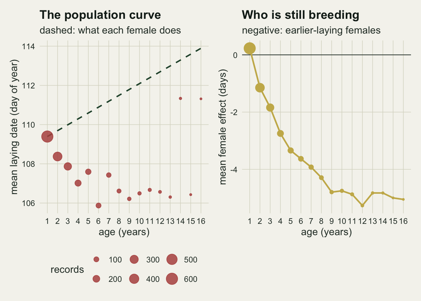
Selective disappearance and the repair
One study is one draw. The chunk below runs forty studies, in five batches of eight, and fits each with nine analyses, eight of which appear in the figure. The first two are the ones the scene above used. The next five use the two individual-level covariates of van de Pol and Verhulst (2006): the age at last reproduction, and the female’s mean age (the within-individual centring, which is the Mundlak form of the within- and between-individual effects post applied to age). Each is fitted as recorded and with a flag for females still breeding in the last season, and the age at last reproduction is also fitted on females whose history is complete. The flag and the restriction deal with the females still alive at the end of the study; they are additions made here, not part of the model the paper sets out. The eighth is the pure within-female estimator, each female’s records centred on her own means, with no season term at all. The ninth is described below.
fit_age <- function(fml, dat)
  fixef(lme(fml, random = ~ 1 | fid, data = dat, control = ctl))[["age"]]
sel_study <- function() {
  d <- sim_study(A = a_lin, beta_sel = beta_sel)
  d$entered_old <- as.numeric(ave(d$age, d$id, FUN = min) > 1)   # first recorded older than one
  d_dead <- d[d$alive_end == 0, ]
  d_mlay <- ave(d$lay, d$id)
  c(population = coef(lm(lay ~ age + fyear, data = d))[["age"]],
    naive      = fit_age(lay ~ age + fyear, d),
    alr        = fit_age(lay ~ age + alr + fyear, d),
    alr_flag   = fit_age(lay ~ age + alr + alive_end + fyear, d),
    alr_dead   = fit_age(lay ~ age + alr + fyear, d_dead),
    mage       = fit_age(lay ~ age + mage + fyear, d),
    mage_flag  = fit_age(lay ~ age + mage + alive_end + fyear, d),
    within     = sum((d$age - d$mage) * (d$lay - d_mlay)) / sum((d$age - d$mage)^2),
    mage_entry = fit_age(lay ~ age + mage + alive_end + entered_old + fyear, d))
}
n_draw <- 5; n_per_draw <- 8
set.seed(3302)
sel_raw <- do.call(rbind, lapply(seq_len(n_draw), function(k)
  data.frame(draw = k, t(replicate(n_per_draw, sel_study())))))
mods <- setdiff(names(sel_raw), "draw")
mods_fig <- setdiff(mods, "mage_entry")     # the ninth fit is reported in the text only
draw_med <- aggregate(sel_raw[, mods], by = list(draw = sel_raw$draw), FUN = median)
sel_sum <- data.frame(model = mods,
  med  = sapply(mods, function(m) median(draw_med[[m]])),
  lo   = sapply(mods, function(m) min(draw_med[[m]])),
  hi   = sapply(mods, function(m) max(draw_med[[m]])),
  mean = colMeans(sel_raw[, mods]),
  sdev = apply(sel_raw[, mods], 2, sd),
  mcse = apply(sel_raw[, mods], 2, sd) / sqrt(nrow(sel_raw)))
st <- function(m, col = "med") sel_sum[m, col]
n_studies <- nrow(sel_raw)
naive_z  <- (st("naive", "mean") - a_lin) / st("naive", "mcse")
closer_draws <- sum(abs(draw_med$alr - a_lin) < abs(draw_med$naive - a_lin))
z_of <- function(m) (st(m, "mean") - a_lin) / st(m, "mcse")
The numbers below are the median of the five batch medians, with the range of the batch medians in brackets. The regression with no female term gives -0.160 [-0.208, -0.131] days per year of age; the random intercept model gives +0.065 [+0.039, +0.089]. The truth is +0.3. Over all 40 studies the random intercept slope averages +0.063 with a Monte Carlo standard error of 0.006, 38 standard errors from the truth. The random intercept soaks up part of the difference among females, not all of it, because the model assumes the female effects are unrelated to age and selection makes them related.
Adding the age at last reproduction as it stands in the data moves the slope to +0.388 [+0.359, +0.433], and the mean-age term to +0.403 [+0.384, +0.456]. Both repairs land much closer to the truth than the naive fit did (the covariate version in 5 of 5 batches), and both land past it: their means sit 11.2 and 13.8 Monte Carlo standard errors above 0.3.
The overshoot comes from the females that outlived the study. For them the recorded age at last reproduction and the mean age are cut off by the last season, so a good female hatched late in the study looks, on the covariate, like a poor female that died young. Give those females a flag, one extra column, and the slope comes back to +0.306 [+0.287, +0.340] with the age at last reproduction, a mean 1.4 Monte Carlo standard errors from the truth, and +0.322 [+0.305, +0.345] with the mean age, still a little high at 2.4 standard errors. The remaining excess comes from the other end of the study: females hatched before the first season enter it at older ages, which raises their mean age over their records but not their age at last reproduction. The ninth fit adds a second flag, for females first recorded older than one, to the mean-age model, and its slope is +0.301 [+0.287, +0.320], a mean 0.3 Monte Carlo standard errors from the truth. The other common choice, fitting only females whose life history is complete, gives +0.308 [+0.280, +0.322] (a mean of +0.300, Monte Carlo standard error 0.010), at the price of the records of the 15 per cent or so of females still alive. Why a censored covariate matters this much is the subject of the last section: with seasons as a factor, the change in a female’s age from one season to the next is also the change in season, so the slope has to be read from females of different hatch years breeding in the same season, and that comparison is only as clean as the covariate that describes them.
The pure within-female estimator, which ignores seasons altogether, averages +0.333 (Monte Carlo standard error 0.024), unbiased as far as forty studies can tell. Its cost shows in the spread: the standard deviation across studies is 0.152, against 0.042 for the flagged covariate model. Without a season term each study’s slope carries whatever trend its own twenty season effects happen to have, and in a real population, where seasons trend with climate, that trend is not noise.
mod_lab <- c(population = "no female term",
             naive      = "age + (1 | female)",
             alr        = "+ last breeding age, as recorded",
             alr_flag   = "+ last breeding age + still-breeding flag",
             alr_dead   = "+ last breeding age, dead females only",
             mage       = "+ mean age, as recorded",
             mage_flag  = "+ mean age + still-breeding flag",
             within     = "within female only, no season term")
mod_grp <- c(population = "ignores selection", naive = "ignores selection",
             alr = "repair, censoring ignored", mage = "repair, censoring ignored",
             alr_flag = "repair, censoring handled", mage_flag = "repair, censoring handled",
             alr_dead = "repair, censoring handled", within = "no season term")
long_sel <- data.frame(model = rep(mods_fig, each = n_studies),
                       est = unlist(sel_raw[, mods_fig], use.names = FALSE))
long_sel$label <- factor(mod_lab[long_sel$model], levels = rev(mod_lab))
long_sel$group <- factor(mod_grp[long_sel$model], levels = unique(mod_grp))
med_sel <- aggregate(est ~ label, data = long_sel, FUN = median)
ggplot(long_sel, aes(est, label, colour = group, shape = group)) +
  geom_vline(xintercept = a_lin, colour = te_forest, linetype = "dashed", linewidth = 0.7) +
  geom_vline(xintercept = 0, colour = te_body, linetype = "dotted", linewidth = 0.5) +
  geom_point(position = position_jitter(height = 0.15, width = 0, seed = 1),
             size = 1.4, alpha = 0.65) +
  geom_errorbar(data = med_sel, aes(xmin = est, xmax = est, y = label), inherit.aes = FALSE,
                width = 0.6, linewidth = 1.1, colour = te_ink) +
  scale_colour_manual(values = c(te_rust, te_gold, te_forest, te_body), name = NULL) +
  scale_shape_manual(values = c(16, 16, 16, 1), name = NULL) +
  guides(colour = guide_legend(nrow = 2), shape = guide_legend(nrow = 2)) +
  labs(x = "linear ageing slope (days per year of age)", y = NULL,
       title = "Selective disappearance and its repair",
       subtitle = "dashed: the true within-female slope") +
  theme_datasheet() + theme(legend.position = "bottom")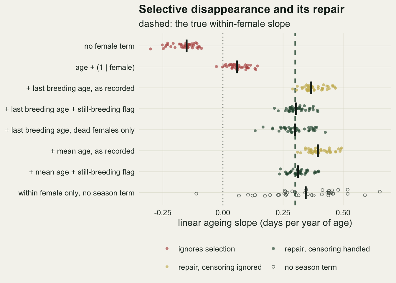
Onset, curvature and the prime age
A linear slope is the simplest summary and rarely the right one. Young females lay late, females in their prime lay early, and old females lay late again, so the age pattern has a minimum, the prime age, and senescence is what happens after it. The usual model adds a quadratic term in age; the prime age is then minus the linear coefficient divided by twice the quadratic one. The next scenario has no selection and no trend across hatch years: the age term in laying date is minus 1.2 days times age plus 0.12 days times age squared, so the earliest laying is at age five, and the question is how well a study of ten, twenty or forty seasons recovers that age.
a_q <- -1.2; q_q <- 0.12            # quadratic age curve, earliest laying at age 5
prime_true <- -a_q / (2 * q_q)
len_grid <- c(10, 20, 40); n_len <- 30
quad_fit <- function(d) {
  f <- fixef(lme(lay ~ age + I(age^2) + fyear, random = ~ 1 | fid, data = d, control = ctl))
  c(a = f[["age"]], q = f[["I(age^2)"]], prime = -f[["age"]] / (2 * f[["I(age^2)"]]))
}
set.seed(3303)
prime_tab <- do.call(rbind, lapply(len_grid, function(ny) do.call(rbind, lapply(seq_len(n_len), function(i) {
  d <- sim_study(A = a_q, Q = q_q, n_seasons = ny)
  data.frame(seasons = ny, n_rec = nrow(d), n_old = sum(d$age >= 8), t(quad_fit(d)))
}))))
pq <- function(ny, p) unname(quantile(prime_tab$prime[prime_tab$seasons == ny], p))
pm <- function(ny, col) median(prime_tab[[col]][prime_tab$seasons == ny])
within1 <- function(ny) mean(abs(prime_tab$prime[prime_tab$seasons == ny] - prime_true) <= 0.5)
With the quadratic as the true shape the answer is reassuring. At twenty seasons the median prime age over 30 studies is 4.97 and the middle 80 per cent of estimates run from 4.39 to 5.46; 73 per cent of studies put it within half a year of 5. Ten seasons widen that range to 4.35 to 6.71, and forty narrow it to 4.69 to 5.35. The limit is the old females: a twenty-season study has a median of 79 records from females aged eight or more, out of 1708.
That reassurance rests on the quadratic being the true shape, and a quadratic is symmetric about its minimum. The second arm keeps everything else and replaces the curve with a broken stick: laying advances by 1.5 days per year until age three and then gets later by 0.6 days per year, so the prime age and the onset of senescence are both three. Each study is fitted with the quadratic and with a broken stick whose knot is chosen by maximum likelihood among the integer ages two to six (ages are whole years, so an integer grid is the natural one; the fits use maximum likelihood rather than REML because the fixed-effect columns change with the knot).
knot_true <- 3; b_before <- -1.5; b_after <- 0.6
knot_grid <- 2:6
stick_fit <- function(d, k) {
  d$pre <- pmin(d$age, k); d$post <- pmax(d$age - k, 0)
  m <- lme(lay ~ pre + post + fyear, random = ~ 1 | fid, data = d, control = ctl, method = "ML")
  c(ll = as.numeric(logLik(m)), before = fixef(m)[["pre"]], after = fixef(m)[["post"]])
}
set.seed(3304)
arm_tab <- do.call(rbind, lapply(seq_len(n_len), function(i) {
  d <- sim_study()
  d$lay <- d$lay + b_before * pmin(d$age, knot_true) + b_after * pmax(d$age - knot_true, 0)
  qf <- quad_fit(d)
  sf <- sapply(knot_grid, function(k) stick_fit(d, k))
  best <- which.max(sf["ll", ])
  data.frame(q_prime = qf[["prime"]], q_slope9 = qf[["a"]] + 2 * qf[["q"]] * 9,
             knot = knot_grid[best], before = sf["before", best], after = sf["after", best])
}))
knot_hit <- mean(arm_tab$knot == knot_true)
The quadratic puts the prime age at a median of 4.96 (range 4.25 to 6.14), 2.0 years after the real onset, and its slope at age nine has a median of 0.95 days per year against a true 0.6. The broken stick finds the knot at 3 in 97 per cent of studies, and its slope after the knot has a median of 0.59. The quadratic is not wrong as a smoother; it is wrong as a statement about when senescence starts, because its minimum is wherever symmetry puts it.
prime_tab$len_lab <- factor(sprintf("%d seasons", prime_tab$seasons),
                            levels = sprintf("%d seasons", len_grid))
med_len <- aggregate(prime ~ len_lab, data = prime_tab, FUN = median)
p_len <- ggplot(prime_tab, aes(len_lab, prime)) +
  geom_hline(yintercept = prime_true, colour = te_forest, linetype = "dashed", linewidth = 0.7) +
  geom_point(position = position_jitter(width = 0.15, height = 0, seed = 2),
             colour = te_gold, size = 1.6, alpha = 0.8) +
  geom_errorbar(data = med_len, aes(x = len_lab, ymin = prime, ymax = prime),
                width = 0.5, linewidth = 1.1, colour = te_ink) +
  labs(x = NULL, y = "estimated prime age (years)", title = "Quadratic truth",
       subtitle = "dashed: true prime age") +
  theme_datasheet()
arm_long <- data.frame(fit = factor(rep(c("quadratic: prime age", "broken stick: knot"),
                                        each = nrow(arm_tab)),
                                    levels = c("quadratic: prime age", "broken stick: knot")),
                       age = c(arm_tab$q_prime, arm_tab$knot))
med_arm <- aggregate(age ~ fit, data = arm_long, FUN = median)
p_arm <- ggplot(arm_long, aes(fit, age, colour = fit)) +
  geom_hline(yintercept = knot_true, colour = te_forest, linetype = "dashed", linewidth = 0.7) +
  geom_point(position = position_jitter(width = 0.15, height = 0.05, seed = 3),
             size = 1.6, alpha = 0.8) +
  geom_errorbar(data = med_arm, aes(x = fit, ymin = age, ymax = age), inherit.aes = FALSE,
                width = 0.5, linewidth = 1.1, colour = te_ink) +
  scale_colour_manual(values = c(te_rust, te_forest), guide = "none") +
  labs(x = NULL, y = "estimated age (years)", title = "Broken-stick truth",
       subtitle = "dashed: true onset and prime age") +
  theme_datasheet()
p_len + p_arm + plot_annotation(theme = theme_datasheet())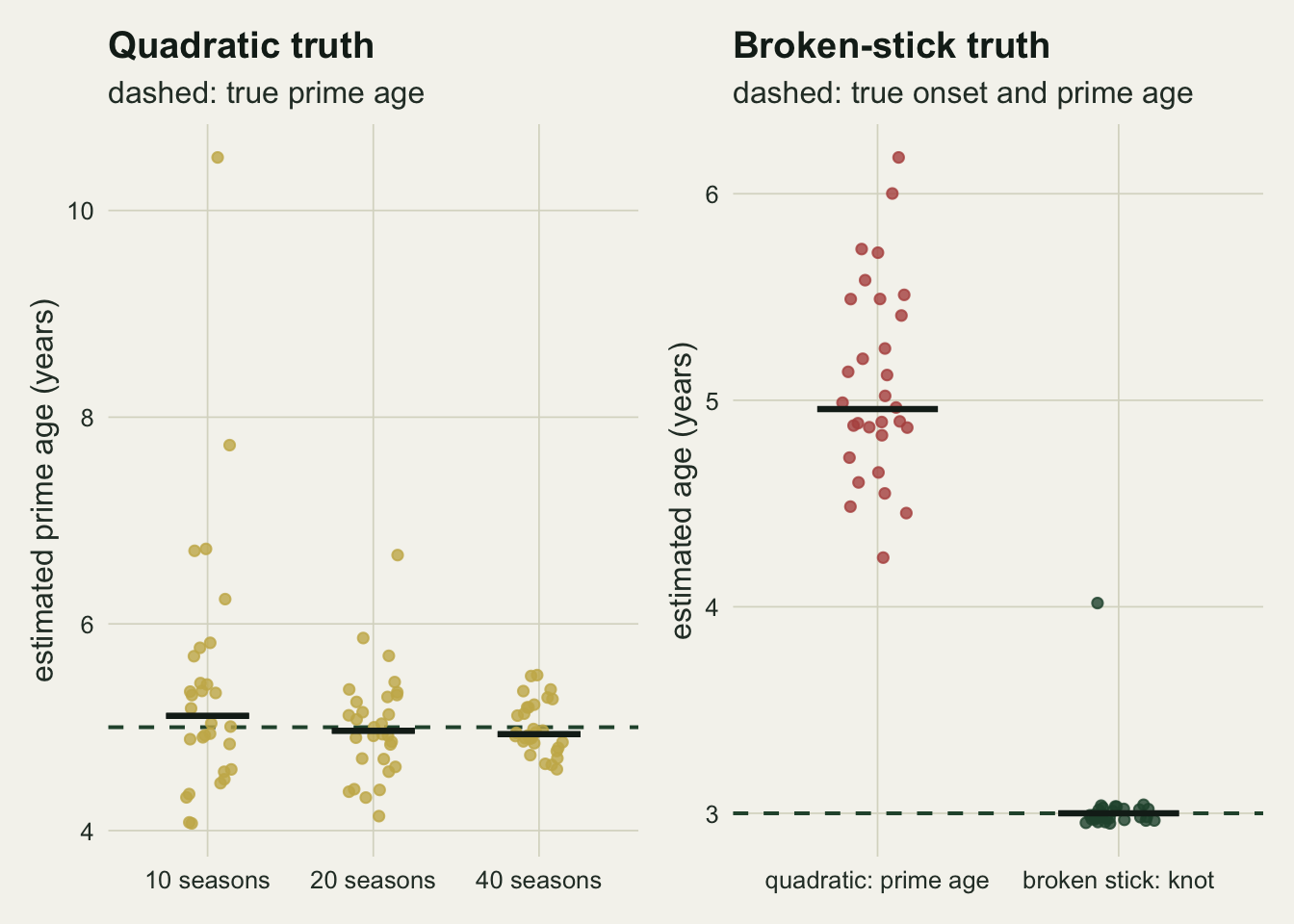
Age, season and hatch year: one column too many
Everything so far had no trend across hatch years. Suppose there is one: each successive hatch year lays 0.3 days earlier throughout life, because natal conditions improved or because the population is responding to selection. Every record satisfies age = season minus hatch year, so a term C times hatch year can be rewritten as C times season minus C times age:
\[\text{lay} = f(\text{age}) + C\,\text{hatch} + \dots = \big(f(\text{age}) - C\,\text{age}\big) + C\,\text{season} + \dots\]
A season factor absorbs C times season completely, and the age function is left with an extra straight line of slope minus C. The linear age coefficient becomes A - C; the quadratic coefficient Q does not move; the prime age moves from -A / (2Q) to -(A - C) / (2Q), a shift of C / (2Q). This is Holford’s (1983) identity for age, period and cohort, and in this model it is exact rather than approximate. The added column lies inside the space spanned by the fixed effects, so the residuals, and with them the REML estimates of the variance components, are unchanged; the fixed effects shift by exactly the added coefficients. The chunk below checks that on one simulated study by fitting it twice, once as simulated and once with the hatch-year trend added to the same laying dates.
c_trend <- -0.3                      # days per hatch year; later hatch years lay earlier
set.seed(3305)
base  <- sim_study(A = a_q, Q = q_q)
trend <- base; trend$lay <- base$lay + c_trend * base$cohort
fit_pair <- function(d) {
  m1 <- lme(lay ~ age + I(age^2) + fyear, random = ~ 1 | fid, data = d, control = ctl)
  m2 <- lme(lay ~ age + I(age^2) + fyear, random = ~ 1 | fcoh / fid, data = d, control = ctl)
  c(a1 = fixef(m1)[["age"]], q1 = fixef(m1)[["I(age^2)"]],
    a2 = fixef(m2)[["age"]], q2 = fixef(m2)[["I(age^2)"]])
}
fp_base <- fit_pair(base); fp_trend <- fit_pair(trend)
fp_diff <- fp_trend - fp_base
prime_b <- -fp_base[["a1"]] / (2 * fp_base[["q1"]])
prime_t <- -fp_trend[["a1"]] / (2 * fp_trend[["q1"]])
prime_formula <- -(a_q - c_trend) / (2 * q_q)
shift_formula <- c_trend / (2 * q_q)
gap_lin  <- max(abs(fp_diff[c("a1", "a2")] - (-c_trend)))
gap_quad <- max(abs(fp_diff[c("q1", "q2")]))
stick_base  <- sapply(knot_grid, function(k) stick_fit(base, k))
stick_trend <- sapply(knot_grid, function(k) stick_fit(trend, k))
knot_b <- knot_grid[which.max(stick_base["ll", ])]
knot_t <- knot_grid[which.max(stick_trend["ll", ])]
gap_ll <- max(abs(stick_trend["ll", ] - stick_base["ll", ]))
change_b <- stick_base["after", ] - stick_base["before", ]
change_t <- stick_trend["after", ] - stick_trend["before", ]
gap_change <- max(abs(change_t - change_b))
gap_seg <- max(abs(c(stick_trend["before", ] - stick_base["before", ],
                     stick_trend["after", ] - stick_base["after", ]) - (-c_trend)))
Refitting with the hatch-year trend changes the linear age coefficient by +0.3000 in the model with a female random intercept and by +0.3000 in the model with hatch year and female as nested random intercepts, against +0.3 from the algebra; the largest departure is \(1.8 \times 10^{-9}\). The quadratic coefficient moves by at most \(2.2 \times 10^{-10}\). The prime age goes from 4.60 to 3.36 in this study; with the true coefficients the same formula takes it from 5.00 to 3.75, a shift of -1.25 years. The random intercept for hatch year does not help, and cannot: the trend lies in the space of columns the fixed part already spans, season and age, so whatever the random effects, the fit puts it there, in the age column.
The broken stick behaves the same way. Across the five candidate knots its maximised log-likelihood changes by at most \(1.5 \times 10^{-10}\), so the chosen knot is the same (4 before, 4 after; these data were simulated with the quadratic, so the knot is only the best-fitting corner). Both segment slopes move by +0.3, to within \(2.9 \times 10^{-8}\) at every knot, and the change in slope at the knot moves by at most \(3.5 \times 10^{-8}\). With a season factor in the model, whatever part of the age pattern is a straight line cannot be told apart from a linear trend across hatch years; every departure from a straight line can be, as long as the hatch-year trend is itself a straight line. For the quadratic that is Q; for the broken stick it is the knot and the change of slope at it; for a smooth it is the shape up to an added straight line. The prime age of a quadratic depends on the linear coefficient, so it is not identified; the knot of a broken stick does not, so it is, for as long as the broken stick is the right shape.
age_seq <- seq(1, 12, by = 0.1)
curve_rel <- function(a, q) a * (age_seq - 1) + q * (age_seq^2 - 1)
curve_dat <- rbind(
  data.frame(age = age_seq, rel = curve_rel(a_q, q_q), fit = "true curve"),
  data.frame(age = age_seq, rel = curve_rel(fp_base[["a1"]], fp_base[["q1"]]), fit = "fitted, as simulated"),
  data.frame(age = age_seq, rel = curve_rel(fp_trend[["a1"]], fp_trend[["q1"]]), fit = "fitted, hatch-year trend added"))
curve_dat$fit <- factor(curve_dat$fit, levels = c("true curve", "fitted, as simulated",
                                                  "fitted, hatch-year trend added"))
prime_pts <- data.frame(age = c(prime_b, prime_t),
                        rel = c(fp_base[["a1"]] * (prime_b - 1) + fp_base[["q1"]] * (prime_b^2 - 1),
                                fp_trend[["a1"]] * (prime_t - 1) + fp_trend[["q1"]] * (prime_t^2 - 1)),
                        fit = factor(c("fitted, as simulated", "fitted, hatch-year trend added"),
                                     levels = levels(curve_dat$fit)))
fig_identity <- ggplot(curve_dat, aes(age, rel, colour = fit, linetype = fit)) +
  geom_line(linewidth = 1) +
  geom_point(data = prime_pts, size = 3, show.legend = FALSE) +
  scale_colour_manual(values = c(te_body, te_forest, te_rust), name = NULL) +
  scale_linetype_manual(values = c("dashed", "solid", "solid"), name = NULL) +
  scale_x_continuous(breaks = 1:12) +
  guides(colour = guide_legend(nrow = 2)) +
  labs(x = "age (years)", y = "laying date relative to age one (days)",
       title = "Same curvature, different prime age",
       subtitle = "the hatch-year trend enters as a straight line in age") +
  theme_datasheet() + theme(legend.position = "bottom")
fig_identity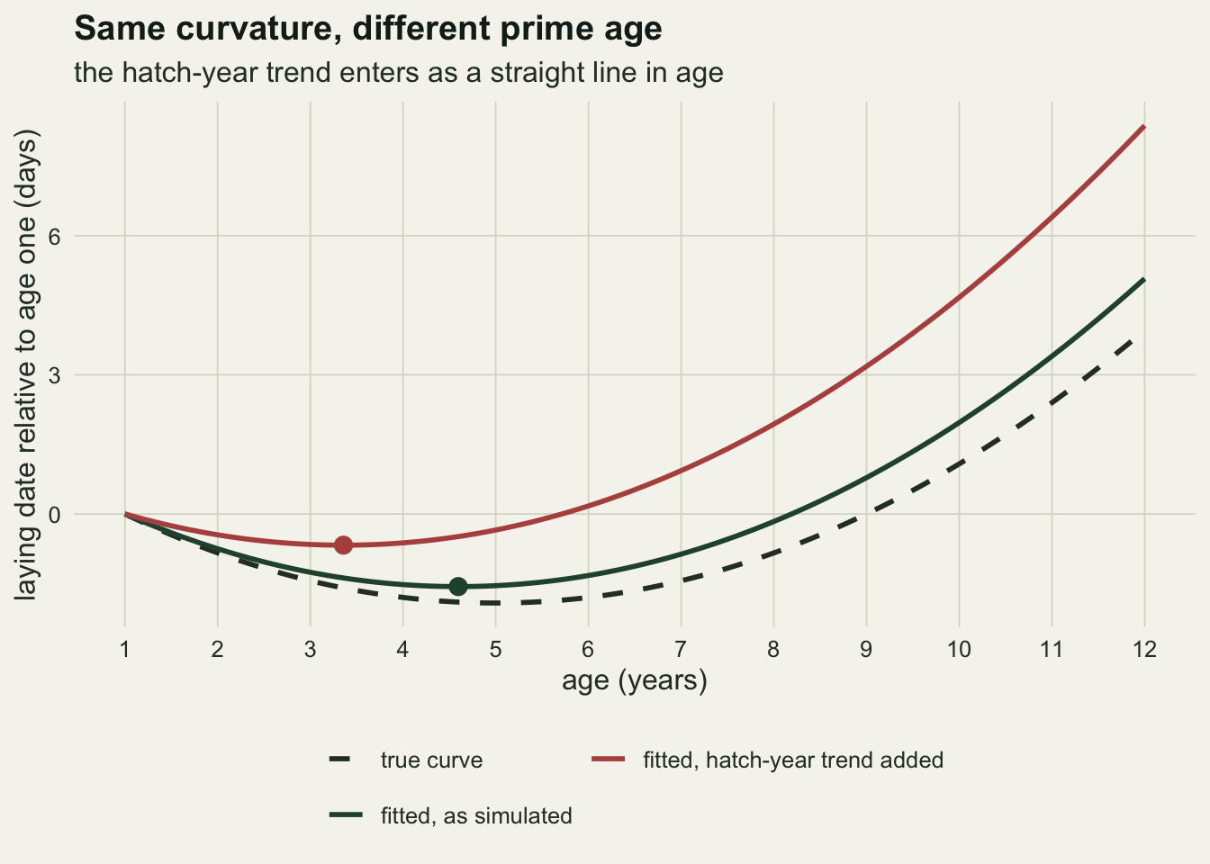
Ordinary least squares makes the same point more bluntly. With female and season both as fixed factors, age is an exact linear combination of the other columns, and lm does not stop; it drops whichever aliased column comes last in the formula.
lm_age_first <- coef(lm(lay ~ age + fyear + fid, data = base))
lm_age_last  <- coef(lm(lay ~ fyear + fid + age, data = base))
n_na_first <- sum(is.na(lm_age_first)); age_last_na <- is.na(lm_age_last[["age"]])
Written with age first, the fit reports an age slope of -0.285 and sets 1 female coefficient to NA; written with age last, the age coefficient itself is NA (as it should be). The first number is not an estimate of anything; it is the slope that one arbitrary constraint on the female effects happens to produce. The same kind of arbitrary choice sets the prediction for an empty cell of a crossed design, as Factor levels in R: reference groups and empty sites shows with habitat and season.
What can break the tie is a measured covariate that carries the hatch-year trend, for instance a natal condition index recorded in each hatch year, and only for the part of the trend it carries. Its coefficient is estimated from its departures from its own straight-line trend across hatch years; an index that followed the trend exactly would be aliased with age and season, as hatch year is. The last chunk gives the hatch years such an index, with a trend of its own plus year-to-year noise, and lets it carry all of the hatch-year trend or half of it.
k_nat <- 0.2                         # trend of the natal index per hatch year
nat_z <- k_nat * ((-n_pre):(n_year - 2)) + rnorm(n_year - 1 + n_pre)
base$natal <- nat_z[base$cohort + n_pre + 1]
natal_age <- function(s) {
  d <- base
  d$lay <- base$lay + (1 - s) * c_trend * base$cohort + s * (c_trend / k_nat) * base$natal
  fixef(lme(lay ~ age + natal + fyear, random = ~ 1 | fid, data = d, control = ctl))[["age"]]
}
nat_0 <- natal_age(0)
nat_ref <- fixef(lme(lay ~ age + natal + fyear, random = ~ 1 | fid, data = base, control = ctl))[["age"]]
shift_full <- natal_age(1) - nat_ref; shift_half <- natal_age(0.5) - nat_ref
shift_none <- nat_0 - nat_ref
With the index in the model, a hatch-year effect carried entirely by the index shifts the linear age coefficient by \(6.1 \times 10^{-9}\); carried half by the index and half by an unmeasured trend it shifts it by +0.150, and with no help from the index by +0.300. The rule is again exact: the index removes the part of the hatch-year effect that is a linear function of the index, and the linear trend in whatever is left goes into the age slope. An index measured with error would remove less, by the usual attenuation.
What to report
Fit ageing within individuals with an individual-level selection term, as van de Pol and Verhulst (2006) describe: the age at last reproduction, or the individual’s mean age. Say how individuals still alive at the end of the study were treated. In the design here, treating their last recorded age as a last breeding age pushed the slope past the truth by 0.09 days per year, and either a still-breeding flag or a restriction to complete histories removed most of that.
Report the curvature, and for a broken stick the knot and the change in slope at it, with their intervals. These are identified whatever the linear trend across hatch years. Say which shape was fitted and why; a quadratic prime age on a curve that is not symmetric is a statement about the quadratic.
Do not report a linear ageing slope, or a prime age from a quadratic, from a model with season effects unless the assumption that makes them identified is written down: that there is no linear trend across hatch years in the quantity being modelled. Where that assumption is doubtful, measure the natal conditions that could carry such a trend and put them in the model. A random intercept for hatch year is not that measurement. The review of Fosse and Winship (2019) covers the options outside ecology, including bounds on the linear components, for readers who need more than a stated assumption.
Give the design next to the numbers: seasons, recruits per year, the share of records from old individuals, and the share of individuals censored at the end. In the twenty-season design here, a quadratic prime age was pinned to within half a year in 73 per cent of studies, against 53 per cent at ten seasons and 97 per cent at forty.
Honest limits
Every female breeds every year from age one until she dies, and every attempt is recorded. Real studies miss breeding attempts, lose females to emigration and see first breeding at different ages; Nussey et al. (2008) discuss capture-mark-recapture models for the detection part, and van de Pol and Verhulst (2006) add an age at first reproduction term for the recruitment part, which this simulation cannot exercise because every female recruits at the same age. Terminal effects, a drop in performance in the last season before death, are not simulated either; they are commonly fitted as a separate indicator for the final attempt, which for females still alive at the end of the study is again unknown.
Selection acts only through survival, on the female’s intercept, with a strength fixed at one on the log odds scale per standard deviation. Weaker selection should give a smaller naive bias; no attempt was made to find the strength at which it disappears. Females all age at the same rate; with individual differences in ageing, a random slope on age is needed, and the between-female covariates then have a second job.
The overshoot of the raw covariates and its repair by a flag or by complete histories were measured in one design, in which 15 per cent of the females of the example study outlived it. A longer-lived species, or a shorter study, censors more females, and the size of the overshoot should be expected to change with that share. The flag was the simplest fix that worked here, not a general recommendation.
The identity in the last section is exact for linear trends and for the fixed-effect and nested random-effect models fitted here. Seasons as a random effect were not fitted. With many records per season the season effects are barely shrunk, so such a model should behave almost like the season factor and give nearly all of a hatch-year trend to the age slope; it is not an escape from the identity. The natal index was measured without error; with error it removes only part of the trend.
References
Holford TR 1983 Biometrics 39(2):311 (10.2307/2531004)
van de Pol M, Verhulst S 2006 American Naturalist 167(5):766-773 (10.1086/503331)
Nussey DH, Coulson T, Festa-Bianchet M, Gaillard JM 2008 Functional Ecology 22(3):393-406 (10.1111/j.1365-2435.2008.01408.x)
Fosse E, Winship C 2019 Annual Review of Sociology 45:467-492 (10.1146/annurev-soc-073018-022616)