library(dplyr)
library(ggplot2)
options(scipen = 6)   # print small p-values as decimals

te_paper  <- "#f5f4ee"
te_ink    <- "#16241d"
te_body   <- "#2c3a31"
te_forest <- "#275139"
te_rust   <- "#b5534e"
te_gold   <- "#c9b458"
te_line   <- "#dad9ca"

theme_datasheet <- function() {
  theme_minimal(base_size = 12) +
    theme(plot.background  = element_rect(fill = te_paper, colour = NA),
          panel.background = element_rect(fill = te_paper, colour = NA),
          panel.grid.major = element_line(colour = te_line, linewidth = 0.3),
          panel.grid.minor = element_blank(),
          text             = element_text(colour = te_body),
          axis.text        = element_text(colour = te_body),
          strip.text       = element_text(colour = te_ink, face = "bold"))
}Factor levels in R: reference groups and empty sites
R
dplyr
data wrangling
data cleaning
regression
ecology tutorial
Factor levels in R decide which group a model compares against and which sites vanish from a count. Set them from the design, keep empty sites, catch stray NAs.
A fire experiment: quadrats that were left alone, quadrats that were burnt, quadrats that were mown, and the dry biomass cut from each at the end of the season. You fit lm(biomass ~ treatment), open the coefficient table, and there is a row for treatmentcontrol but no row for burnt. Nothing failed. R has made a choice about your treatment column, and the table is an answer to a question you did not ask.
A factor is R’s way of storing a grouping column: a set of labels plus a list of the allowed values, the levels, in a fixed order. That list decides three things that show up in ecological results. Its first entry is the group every model coefficient is measured against. Its members are the groups that a count or a summary is allowed to report, including groups with nothing in them. And any value that is not on the list stops being a value at all. Each of the three main sections below runs one of these on a small simulated data set, shows the number that comes out wrong without any warning, and then fixes it. Two further sections add the cases next to them: an empty cell in a crossed design, where R does warn but quietly, and a grouping column stored as numbers, which never becomes a factor at all.
The short answer. Turn every grouping column into a factor yourself, with the levels written out from your study design rather than taken from the data. Put the group you want to compare against first. Include the sites that produced no records. Then check that no value dropped out on the way.
This post assumes you have met group_by() and summarise(), which Summarising ecological data by group introduces. The data are simulated, and every seed is in the code.
The first level is the reference group
Eight quadrats per treatment, with true mean biomass fixed in the code at 120 g for control, 90 g for burnt and 95 g for mown: mowing is built to remove almost as much as fire does. The treatment column is plain text, which is what read.csv() and data.frame() give you: since R 4.0.0 neither turns text into factors unless you ask.
set.seed(1012)
treat_means <- c(control = 120, burnt = 90, mown = 95)    # true means, g per quadrat
n_per <- 8

plots <- data.frame(treatment = rep(names(treat_means), each = n_per))
plots$biomass <- round(rnorm(nrow(plots), mean = treat_means[plots$treatment], sd = 15), 1)

stopifnot(is.character(plots$treatment),
          is.character(read.csv(text = "treatment\nburnt")$treatment))
head(plots, 3)
treatment biomass
1 control 107.9
2 control 117.5
3 control 111.5lm() needs groups, so it converts the text column to a factor on the way in. factor() sorts the distinct values to make the levels, the first sorted level becomes the reference, and “burnt” comes before “control” in the alphabet.
stopifnot(identical(levels(factor(plots$treatment)), c("burnt", "control", "mown")))

fit_default <- lm(biomass ~ treatment, data = plots)
cf_def <- coef(summary(fit_default))
round(cf_def, 4)
Estimate Std. Error t value Pr(>|t|)
(Intercept) 88.9500 5.1737 17.1927 0.0000
treatmentcontrol 37.8000 7.3167 5.1662 0.0000
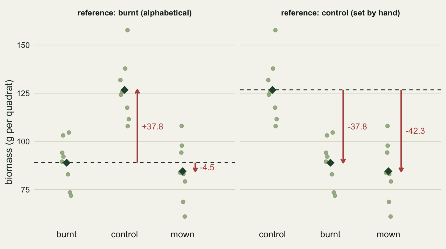
treatmentmown -4.4875 7.3167 -0.6133 0.5463Read the table the way the model means it. The intercept, 89.0 g, is the mean of the burnt quadrats. treatmentcontrol is control minus burnt, +37.8 g. And treatmentmown is mown minus burnt: -4.5 g with a p-value of 0.55. Read as “the effect of mowing”, that row says mowing did very little. It says nothing of the sort. It compares two disturbance treatments with each other, and the comparison the experiment was built for, mown against untouched, is not in the table at all.
The fix is one line. Make the column a factor and name the reference, either with relevel() or by writing out all the levels in the order you want (useful later for plots and tables):
plots$treatment <- relevel(factor(plots$treatment), ref = "control")
# same result: factor(plots$treatment, levels = c("control", "burnt", "mown"))
levels(plots$treatment)
[1] "control" "burnt" "mown" fit_control <- lm(biomass ~ treatment, data = plots)
round(coef(summary(fit_control)), 4) Estimate Std. Error t value Pr(>|t|)
(Intercept) 126.7500 5.1737 24.4988 0
treatmentburnt -37.8000 7.3167 -5.1662 0
treatmentmown -42.2875 7.3167 -5.7796 0Now the intercept is the control mean, 126.8 g, and each row is a treatment against it: burnt -37.8 g, mown -42.3 g with a p-value below 0.0001. The same word, mown, sat on a row with a small estimate and a large p-value a moment ago, and now sits on a row with a large negative estimate. relevel() only works on a factor; on a text column it stops with an error, which is why the factor() call comes first.
Nothing about the model itself has changed. The coefficients are differences between the same three group means, taken from a different starting group. (How a factor becomes an intercept plus differences is in t-tests and ANOVA as linear models in R.)
all.equal(fitted(fit_default), fitted(fit_control))[1] TRUEmax_fit_diff <- max(abs(fitted(fit_default) - fitted(fit_control)))
round(c(logLik_default = as.numeric(logLik(fit_default)),
logLik_control = as.numeric(logLik(fit_control)),
r2_default = summary(fit_default)$r.squared,
r2_control = summary(fit_control)$r.squared), 4)logLik_default logLik_control r2_default r2_control
-96.8517 -96.8517 0.6575 0.6575 grp_mean <- tapply(plots$biomass, plots$treatment, mean)
round(grp_mean, 2)control burnt mown
126.75 88.95 84.46 The fitted values of the two models agree to within floating-point rounding. The log-likelihood is -96.8517 both times and R-squared is 0.6575 both times. The reference level changes what each coefficient means; it does not change the fit, the predictions or any test of the treatment as a whole (the next section shows one exception for the predictions: an empty cell in a crossed design). That is why the mistake is easy to miss: every diagnostic you run on the model looks the same. Contrasts and post-hoc comparisons in R goes on to other codings (sum-to-zero, planned contrasts) and to comparing every pair.
The same levels set the order of groups in plots and tables: alphabetical unless you say otherwise. To sort groups by a statistic instead, for bars in order of their mean, reorder() builds the level order from the data:
levels(reorder(plots$treatment, plots$biomass, FUN = mean))[1] "mown" "burnt" "control"Unless a cell of the design is empty
The reference level did not change any prediction above because every treatment had quadrats in it, so every prediction was the mean of quadrats that were cut. With two grouping columns crossed, that can fail. A second survey cuts biomass in three habitats in three seasons, four quadrats for each habitat and season, except that the wetland was under water in spring and its quadrats were never cut. The true means are fixed in the code, with a wetland that is poor in spring and peaks in autumn.
set.seed(1015)
cell_mean <- rbind(forest    = c(spring = 60, summer =  80, autumn =  70),   # true means, g
                   grassland = c(spring = 90, summer = 140, autumn = 100),
                   wetland   = c(spring = 70, summer = 130, autumn = 150))
survey <- expand.grid(quadrat = 1:4, season = colnames(cell_mean),
                      habitat = rownames(cell_mean), stringsAsFactors = FALSE)
survey <- subset(survey, !(habitat == "wetland" & season == "spring"))   # flooded, never cut
survey$biomass <- round(rnorm(nrow(survey), cell_mean[cbind(survey$habitat, survey$season)],
                              sd = 15), 1)
table(survey$habitat, survey$season)
            autumn spring summer
  forest         4      4      4
  grassland      4      4      4
  wetland        4      0      4
The model biomass ~ habitat * season asks for a separate mean in every habitat and season, the interaction. Fit it twice: once with the text columns as they are, so forest and autumn are the references because they come first in the alphabet, and once with grassland and summer set as the references by hand. Then ask both fits for the cell that was never cut.
fit_alpha <- lm(biomass ~ habitat * season, data = survey)

survey_hand <- survey
survey_hand$habitat <- factor(survey$habitat, levels = c("grassland", "forest", "wetland"))
survey_hand$season  <- factor(survey$season, levels = c("summer", "spring", "autumn"))
fit_hand <- lm(biomass ~ habitat * season, data = survey_hand)

wet_spring <- data.frame(habitat = "wetland", season = "spring")
pred_alpha <- suppressWarnings(predict(fit_alpha, wet_spring))   # the warning is shown below
pred_hand  <- suppressWarnings(predict(fit_hand, wet_spring))
round(c(forest_autumn_first = as.numeric(pred_alpha),
        grassland_summer_first = as.numeric(pred_hand)), 2)
forest_autumn_first grassland_summer_first
132.85 64.15 Both fits give the same fitted value for every quadrat that was cut, and they still predict 132.85 g and 64.15 g for wetland in spring, a cell built at 70 g. Neither number comes from a wetland quadrat in spring, because there are none. Each is put together from three cells that were cut: the wetland mean in the reference season, plus the reference habitat in spring, minus the reference habitat in the reference season. For the alphabetical fit that is wetland in autumn plus forest in spring minus forest in autumn:
cell_avg <- function(h, s) mean(survey$biomass[survey$habitat == h & survey$season == s])
three_cells <- cell_avg("wetland", "autumn") + cell_avg("forest", "spring") - cell_avg("forest", "autumn")
round(c(three_cells = three_cells, alphabetical_fit = as.numeric(pred_alpha)), 2)
three_cells alphabetical_fit
132.85 132.85 It is the prediction of the alphabetical fit. For the fit set by hand the three cells are wetland in summer plus grassland in spring minus grassland in summer. This is arithmetic, not something the simulation found, and it means the gap between the two predictions is set by how differently the habitats change between seasons, the very thing the interaction was meant to estimate.
R does flag the problem, in three places that are easy to scroll past:
coef(fit_alpha)[is.na(coef(fit_alpha))]habitatwetland:seasonspring
NA grep("singularities", capture.output(summary(fit_alpha)), value = TRUE)[1] "Coefficients: (1 not defined because of singularities)"tryCatch(predict(fit_alpha, wet_spring), warning = conditionMessage)[1] "prediction from rank-deficient fit; attr(*, \"non-estim\") has doubtful cases"An NA coefficient means R dropped a column it could not estimate. Fitting a senescence model to individual records meets one of the same kind, where age is tied to female and season, and the slope R does report is what one arbitrary constraint happens to produce. Since R 4.3.0, predict() on an lm() fit takes rankdeficient = "NA" and returns NA for such a row instead of a number, which is the honest answer here: wetland in spring was not measured.
If a number is needed anyway, fit biomass ~ habitat + season without the interaction. It predicts 104.9 g whatever the reference levels, against the 70 g the cell was built at, because it assumes the wetland differs from the other habitats by the same amount in every season. That is an assumption to state in the methods, and in this simulation it is false by construction. Multilevel post-stratification of records fills the empty cells of a survey frame with a main-effects model and with a multilevel model, and measures what each costs.
Sites with no records drop out of a count
A season of camera trapping for pine marten at twenty sites, stored the way detection data usually is: one row per detection. A site where the camera ran all season and saw nothing has no row. Each site’s expected number of detections is drawn at random, so some sites end up empty.
set.seed(1013)
site_ids  <- sprintf("S%02d", 1:20)                 # the survey design
site_rate <- exp(rnorm(length(site_ids), log(1.5), 1))
n_det     <- rpois(length(site_ids), site_rate)

records <- data.frame(site = rep(site_ids, times = n_det))
c(detections = nrow(records), sites_surveyed = length(site_ids),
  sites_with_none = sum(n_det == 0))
detections sites_surveyed sites_with_none
50 20 8 Count detections per site and summarise:
per_site_text <- count(records, site)
c(sites_in_table = nrow(per_site_text),
  mean_detections = mean(per_site_text$n),
  share_detected  = mean(per_site_text$n > 0))
sites_in_table mean_detections share_detected
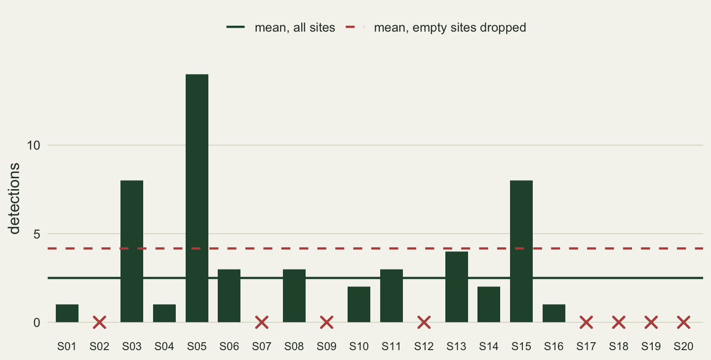
12.000000 4.166667 1.000000 The table has 12 sites, not 20. The 8 sites with no detections are not in records, so no function working from records alone can know they exist. The mean comes out at 4.17 detections per site, and the share of sites where the marten was detected comes out at 1.00: every site in the table has at least one detection, because that is how a site gets into the table.
Turning the column into a factor does not help if the levels come from the same records, since factor() can only list the values it sees: nlevels(factor(records$site)) is 12. The levels have to come from the design, the list of sites you actually surveyed. Even then, count() and group_by() drop empty levels by default, so the argument .drop = FALSE is the second half of the fix:
records$site <- factor(records$site, levels = site_ids)

per_site_default <- count(records, site)
per_site_all     <- count(records, site, .drop = FALSE)

stopifnot(nrow(per_site_default) == sum(n_det > 0),
          nrow(per_site_all) == length(site_ids),
          nrow(count(data.frame(site = as.character(records$site)), site,
                     .drop = FALSE)) == sum(n_det > 0))
c(default = nrow(per_site_default), drop_false = nrow(per_site_all))
default drop_false
12 20 The last line of the stopifnot() is the other half of the rule: .drop = FALSE does nothing for a text column, because a text column has no list of levels to keep. You need both, a factor with the design’s levels and .drop = FALSE. Base R’s table() keeps empty levels without being asked, and group_by() takes the same argument:
sum(table(records$site) == 0)[1] 8per_site <- records |>
group_by(site, .drop = FALSE) |>
summarise(detections = n(), .groups = "drop")
rbind(zeros_dropped = c(sites = nrow(per_site_text), mean = mean(per_site_text$n),
detected = mean(per_site_text$n > 0)),
zeros_kept = c(sites = nrow(per_site), mean = mean(per_site$detections),
detected = mean(per_site$detections > 0))) sites mean detected
zeros_dropped 12 4.166667 1.0
zeros_kept 20 2.500000 0.6With the empty sites back, the mean is 2.50 detections per site and the share of sites with a detection is 0.60. Dropping the zeros inflated the mean by 67 per cent and turned a species detected at 12 of 20 sites into one detected at every site in the table. No simulation is needed for the first number: the same 50 detections are divided by 12 sites instead of 20, so the mean is always inflated by the number of surveyed sites over the number with a detection, minus one (here 20/12 - 1).
The same zeros can come back through a join instead, when the site list lives in its own table; Joining ecological tables without losing zeros takes that route. Either way the site list has to exist somewhere, and it can be lost on the way through a file: What a CSV loses shows an unsampled site disappearing from the level set when a factor is written to CSV and read back.
Levels set by hand turn mismatches into NA
Writing the levels out is the fix in both sections above, and it has a trap of its own. Here is a habitat column for 150 vegetation plots, typed by several people over a season. Most entries are clean, and a few carry a capital letter, a trailing space or a two-word spelling.
set.seed(1014)
n_rec    <- 150
true_hab <- sample(c("forest", "grassland", "wetland"), n_rec, replace = TRUE,
                   prob = c(0.5, 0.3, 0.2))
typed <- true_hab
slip  <- runif(n_rec) < 0.15                         # entries typed differently
variants <- list(forest = c("Forest", "forest "), grassland = c("Grassland", "grassland "),
                 wetland = c("wet land", "Wetland"))
typed[slip] <- vapply(true_hab[slip], function(h) sample(variants[[h]], 1), character(1))
table(typed)
typed
forest Forest forest grassland Grassland grassland wet land
62 4 7 38 3 6 1
wetland Wetland
28 1 You want the habitats in a fixed order, so you write the levels out:
hab_levels <- c("forest", "grassland", "wetland")
habitat <- factor(typed, levels = hab_levels)
c(NA_in_typed = sum(is.na(typed)), NA_in_factor = sum(is.na(habitat)))
NA_in_typed NA_in_factor
0 22 factor() matches each value against the levels exactly, character for character, and every value without a match becomes NA. It does this without a warning. 22 of the 150 plots, 15 per cent of the sheet, now have no habitat, although the column had no missing values a line earlier. The R documentation for factor() states this behaviour; it is not a bug, and nothing downstream will point back to it.
What it does to a class share depends on where the mismatches fall:
round(cbind(true = share_true, after_levels = share_hand,
            plots_lost = lost, plots_left = kept), 3)
true after_levels plots_lost plots_left
forest 0.487 0.484 11 62
grassland 0.313 0.297 9 38
wetland 0.200 0.219 2 28table() leaves NA out unless told otherwise, so every share is now a share of the 128 plots that survived. Wetland lost 2 of its 30 plots, fewer than its fair part of the 22 losses, so its share rose from 0.200 to 0.219 although no wetland plot was added. Grassland lost 9 of its 47, more than its fair part, and its share fell from 0.313 to 0.297. In this simulation every habitat is mistyped at the same rate, so the shares move only a little. When one habitat has a spelling of its own (one recorder who always writes “wet land”) the losses pile up in that class and its share drops with them. The counts are wrong regardless: here every habitat has fewer plots than were surveyed.
The fix is a check before and a check after. Before, ask which values have no level to go to; clean them; ask again:
setdiff(unique(typed), hab_levels)[1] "grassland " "Forest" "Grassland" "forest " "Wetland"
[6] "wet land" cleaned <- tolower(trimws(typed))
setdiff(unique(cleaned), hab_levels)[1] "wet land"cleaned[cleaned == "wet land"] <- "wetland"
habitat <- factor(cleaned, levels = hab_levels)
stopifnot(sum(is.na(habitat)) == sum(is.na(typed)))
all(table(habitat) == table(factor(true_hab, levels = hab_levels)))[1] TRUEtrimws() and tolower() handle the spaces and capitals, and the two-word spelling needs a decision, written down in the code. Cleaning species names before you count does the same job for species names with a lookup table, which scales better than one line per variant. The lasting fix is on the sheet itself: Broman and Woo (2018) make one consistent code per category part of their first rule for spreadsheet data. The stopifnot() after the factor() call is the one to keep in every script: the number of missing values must not change when a column becomes a factor. The forcats package offers fct(), which stops with an error instead of creating NA (chapter 16 of R for Data Science shows the two side by side), if you prefer a loud failure.
One more factor trap is common enough to name: as.numeric() on a factor returns the level positions, not the values. Debugging and defensive R code measures what that does to a regression on elevation.
A grouping column stored as numbers
Field numbers, block numbers and site codes are often typed as 1, 2, 3. R reads such a column as numbers, and a model given numbers fits one straight line through them instead of a separate mean for each group. Say the fire experiment’s 24 quadrats sit in four fields, two quadrats of each treatment in each field, and the fields differ in productivity in an order that has nothing to do with their numbers.
set.seed(1016)
field_effect <- c(0, 40, -30, 20)          # g per quadrat, added in fields 1 to 4
fields <- data.frame(field = rep(1:4, each = 6),
                     treatment = rep(rep(names(treat_means), each = 2), times = 4))
fields$biomass <- round(treat_means[fields$treatment] + field_effect[fields$field] +
                          rnorm(nrow(fields), sd = 15), 1)
str(fields)
'data.frame': 24 obs. of 3 variables:
$ field : int 1 1 1 1 1 1 2 2 2 2 ...
$ treatment: chr "control" "control" "burnt" "burnt" ...
$ biomass : num 131.7 140.6 109.5 92.2 67.6 ...str() shows the problem before any model does: field is int. Fit the treatment test with the field column as it is, and again as a factor:
anova(lm(biomass ~ field + treatment, data = fields))Analysis of Variance Table
Response: biomass
Df Sum Sq Mean Sq F value Pr(>F)
field 1 6.4 6.44 0.0079 0.9299
treatment 2 4672.3 2336.15 2.8749 0.0799 .
Residuals 20 16252.1 812.61
---
Signif. codes: 0 '***' 0.001 '**' 0.01 '*' 0.05 '.' 0.1 ' ' 1anova(lm(biomass ~ factor(field) + treatment, data = fields))Analysis of Variance Table
Response: biomass
Df Sum Sq Mean Sq F value Pr(>F)
factor(field) 3 10664.8 3554.9 11.4392 0.0001977 ***
treatment 2 4672.3 2336.2 7.5174 0.0042336 **
Residuals 18 5593.8 310.8
---
Signif. codes: 0 '***' 0.001 '**' 0.01 '*' 0.05 '.' 0.1 ' ' 1The Df column gives it away: field takes 1 degree of freedom, one slope, and factor(field) takes 3, one difference for each field after the first. A straight line through field effects of 0, 40, -30 and 20 g removes almost none of them (0.2 per cent of their spread), so they stay in the residuals and the treatment test weighs its effect against that extra noise. In this data set the treatment p-value is 0.080 with the numeric field and 0.0042 with the factor. One data set could be luck, so here is the same design drawn 1000 times: with the field effects as above, with the same four effects sorted so that they rise with the field number, and with the four effects put in a new random order for every data set:
p_treatment <- function(effects) {
  y <- treat_means[fields$treatment] + effects[fields$field] + rnorm(nrow(fields), sd = 15)
  c(numeric = anova(lm(y ~ field + treatment, data = fields))["treatment", "Pr(>F)"],
    factor  = anova(lm(y ~ factor(field) + treatment, data = fields))["treatment", "Pr(>F)"])
}
n_sim <- 1000
power_mixed  <- rowMeans(replicate(n_sim, p_treatment(field_effect)) < 0.05)
power_sorted <- rowMeans(replicate(n_sim, p_treatment(sort(field_effect))) < 0.05)
power_random <- rowMeans(replicate(n_sim, p_treatment(sample(field_effect))) < 0.05)
rbind(order_as_above = power_mixed, order_sorted = power_sorted, order_shuffled = power_random)
numeric factor
order_as_above 0.160 0.951
order_sorted 0.953 0.954
order_shuffled 0.391 0.958With the field effects as above, the treatment test found the effect (p below 0.05) in 0.951 of the data sets with factor(field) and in 0.160 with the numeric column. With the effects sorted, the straight line catches nearly all of them, and the factor and the numeric column find the effect in 0.954 and 0.953 of the data sets, the same within Monte Carlo error. The order used above is the worst of the 24 possible orders of these four effects (together with the same order reversed). With the order shuffled for every data set, the numeric column finds the effect in 0.391 of the data sets and the factor in 0.958. (Each share comes from 1000 data sets. Drawn again, a share would typically move by its Monte Carlo standard error, here at most 0.015.) So the damage comes from the order of the codes, and field numbers are labels: nothing makes them line up with productivity, so a numeric column loses power by an amount you cannot know in advance. The trap is for grouping columns in lm(), aov() and glm(). A random effect in lme4, (1 | field), is safe, because lme4 turns the grouping column into a factor itself.
What to check in your own data
Look at levels() of every grouping column before a model sees it, and make sure the first level is the group you want to compare against. If a column is still text when it goes into lm() or glm(), the reference is whatever comes first in the alphabet.
Run str() on the data too. A grouping column listed as int or num (field, block or site numbers) goes into lm() as one slope, not as groups; is.numeric() on every grouping column should be FALSE by the time a model sees it.
Before fitting an interaction of two grouping columns, run table() on the pair; a 0 means a combination the model cannot estimate, and any prediction for it depends on the reference levels.
Write the level list from the design (the sites surveyed, the months sampled, the treatments applied), not from unique() on the records. A site with no records can only appear in a summary if something other than the records knows about it.
When you count or summarise by group, compare the number of rows in the result with the number of groups in the design. If they differ, add .drop = FALSE and check the grouping column is a factor. With .drop = FALSE, an empty group gets n() equal to zero, but mean() of a measurement in that group has nothing to average and returns NaN, so decide what an empty site should show before you plot it.
Every time you call factor() with levels =, run setdiff(unique(x), levels) first and compare the count of NA values before and after. A difference is a spelling you have not dealt with.
Honest limits
Alphabetical order depends on the locale when labels mix capitals and lower case: factor(c("burnt", "Control")) can put either first on different machines, which is one more reason to write the levels out. With two grouping factors, .drop = FALSE keeps every combination of their levels, including combinations the design never had, so check the row count against the design there too.
References
Broman KW, Woo KH 2018 The American Statistician 72(1):2-10 (10.1080/00031305.2017.1375989)
R Core Team 2024 R documentation: Factors (https://stat.ethz.ch/R-manual/R-devel/library/base/html/factor.html)
R Core Team 2024 R documentation: Reorder levels of factor, relevel (https://stat.ethz.ch/R-manual/R-devel/library/stats/html/relevel.html)
Wickham H, Francois R, Henry L, Muller K, Vaughan D 2023 dplyr documentation: Count the observations in each group (https://dplyr.tidyverse.org/reference/count.html)
Wickham H, Cetinkaya-Rundel M, Grolemund G 2023 R for Data Science, 2nd edition, chapter 16: Factors (https://r4ds.hadley.nz/factors.html)