---
title: "Covariates in dynamic occupancy models"
description: "Let colonisation, extinction and detection depend on covariates in base R, and watch a detection covariate leak into the state process when you leave it out."
date: "2026-05-22 11:00"
categories: [occupancy, ecology tutorial, R, population dynamics]
image: thumbnail.png
image-alt: "Two pairs of curves against standardised patch size, each pair a solid fitted line and a dashed truth line, on a per-season rate axis. Colonisation in green rises from near zero to about 0.5; extinction in red falls from about 0.65 to about 0.1. The red pair is widest apart at the left edge, where the dashed truth runs above the fit, then narrows steadily and merges into a single line from about patch size 0.9 rightwards. The green pair stays close throughout, crossing at about patch size 0.6 and ending with the fit a little above the truth."
---
The [basic dynamic occupancy model](../dynamic-occupancy-colonisation-extinction/) treats colonisation, extinction and detection as three numbers that hold for every site and every season. That is a starting point, not an ecology. The questions worth asking are comparative: are large patches colonised more readily, do small patches lose the species faster, is the species harder to detect in dense cover. Each of the three rates can be written as a logit-linear function of covariates, exactly as in an ordinary [logistic regression](../logistic-regression-presence-absence/), and fitted inside the same forward likelihood.
There is a trap waiting in the detection rate. A covariate that raises detection often also correlates with a covariate that shapes the dynamics, and if you model the dynamics but hold detection constant, the detection signal has nowhere to go except into the state process. The result looks like a strong ecological effect and is partly an artefact. This is the multi-season version of the confound in [occupancy with detection covariates](../occupancy-detection-covariates/) and [detection covariates in spatial capture-recapture](../scr-detection-covariates/).
## One covariate on three rates
Take patch size as a standardised site covariate that pushes all three rates. Larger patches are colonised more often, persist better, and (because they hold more individuals and are easier to search) yield higher detection. The three linear predictors are
```
logit(colonisation) = g0 + g1 * size
logit(extinction)   = e0 + e1 * size
logit(detection)    = p0 + p1 * size
```
with `g1 > 0`, `e1 < 0` and `p1 > 0`. That last term is the dangerous one: size and detectability move together.
```{r}
#| label: sim
set.seed(140)
R <- 400; Tn <- 6; K <- 4
size <- as.numeric(scale(runif(R, 0, 1)))
psi1 <- 0.50
g0 <- qlogis(0.18); g1 <-  0.9      # colonisation rises with size
e0 <- qlogis(0.35); e1 <- -0.9      # extinction falls with size
p0 <- qlogis(0.30); p1 <-  0.7      # detection rises with size
gam <- plogis(g0 + g1 * size); ext <- plogis(e0 + e1 * size); pv <- plogis(p0 + p1 * size)

z <- matrix(0L, R, Tn); z[, 1] <- rbinom(R, 1, psi1)
for (t in 2:Tn) z[, t] <- rbinom(R, 1, ifelse(z[, t - 1] == 1, 1 - ext, gam))
d <- matrix(0L, R, Tn); for (t in 1:Tn) d[, t] <- rbinom(R, K, z[, t] * pv)
round(c(mean_gamma = mean(gam), mean_eps = mean(ext), mean_p = mean(pv)), 3)
```
Across sites the average colonisation is 0.214, extinction 0.371 and detection 0.319, so an occupied site is seen at least once in a season about 73 per cent of the time. That gap is enough for the confound to bite.
## Fitting covariates on every rate
The likelihood is the forward pass from the basic model, with the twist that each site now carries its own transition matrix and its own detection probability, built from its covariate value. A single function covers both the correct model and the naive one through a flag that forces detection constant.
```{r}
#| label: likelihood
emit <- function(dt, p, K) c(as.numeric(dt == 0), p^dt * (1 - p)^(K - dt))
site_ll <- function(dv, init, Phi, p, K) {
  a <- init * emit(dv[1], p, K); s <- sum(a); ll <- log(s); a <- a / s
  for (t in 2:length(dv)) {
    a <- as.vector(a %*% Phi) * emit(dv[t], p, K)
    s <- sum(a); ll <- ll + log(s); a <- a / s
  }
  ll
}
mk_nll <- function(p_constant) function(par) {
  ps <- plogis(par[1])
  ga <- plogis(par[2] + par[3] * size); ep <- plogis(par[4] + par[5] * size)
  pvv <- if (p_constant) rep(plogis(par[6]), R) else plogis(par[6] + par[7] * size)
  tot <- 0
  for (i in 1:R) {
    Phi <- matrix(c(1 - ga[i], ga[i], ep[i], 1 - ep[i]), 2, 2, byrow = TRUE)
    tot <- tot + site_ll(d[i, ], c(1 - ps, ps), Phi, pvv[i], K)
  }
  -tot
}
start <- c(0, g0, 0.3, e0, -0.3, p0, 0.3)
fit_full <- optim(start,      mk_nll(FALSE), method = "BFGS", hessian = TRUE)
stopifnot(fit_full$convergence == 0)   # check before inverting the Hessian
se_full  <- sqrt(diag(solve(fit_full$hessian)))
pf <- fit_full$par
round(c(gamma_b1 = pf[3], eps_b1 = pf[5], p_b1 = pf[7],
        se_gamma_b1 = se_full[3], se_eps_b1 = se_full[5], se_p_b1 = se_full[7]), 3)
```
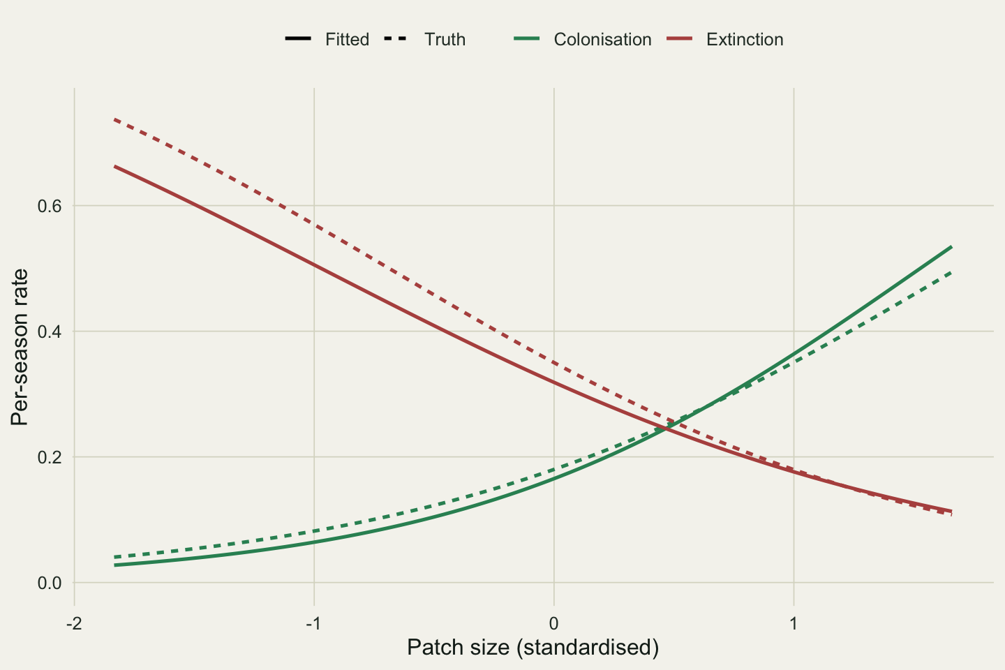
The full model recovers the slopes: colonisation rises with size at 1.06 (SE 0.15), extinction falls at -0.78 (SE 0.14), and detection rises at 0.76 (SE 0.06). All three true values (0.9, -0.9, 0.7) lie within about one standard error. Reading the fitted curves back onto the size axis shows colonisation climbing and extinction dropping across the range of patch sizes.
```{r}
#| label: fig-rates
#| fig-cap: "Fitted per-season colonisation and extinction as functions of patch size, with the true curves dashed. Larger patches are colonised more and go extinct less."
#| fig-alt: "Two curves against standardised patch size. Colonisation in green rises from under 0.05 to about 0.53. Extinction in red falls from about 0.74 to 0.11. Solid fitted lines sit close to dashed truth lines."
#| fig-width: 7.5
#| fig-height: 5.0
suppressMessages({library(ggplot2); library(dplyr)})
theme_te <- function(bs = 12) theme_minimal(base_size = bs) + theme(
  plot.background = element_rect(fill = "#f5f4ee", colour = NA),
  panel.background = element_rect(fill = "#f5f4ee", colour = NA),
  panel.grid.major = element_line(colour = "#dad9ca", linewidth = 0.3),
  panel.grid.minor = element_blank(),
  axis.text = element_text(colour = "#2c3a31"), axis.title = element_text(colour = "#16241d"),
  plot.title = element_text(colour = "#16241d", face = "bold"),
  plot.subtitle = element_text(colour = "#46604a"),
  legend.text = element_text(colour = "#2c3a31"), legend.position = "top",
  legend.key = element_rect(fill = "#f5f4ee", colour = NA))

sg <- seq(min(size), max(size), length = 80)
rate_df <- bind_rows(
  data.frame(size = sg, val = plogis(pf[2] + pf[3] * sg), rate = "Colonisation", kind = "Fitted"),
  data.frame(size = sg, val = plogis(g0 + g1 * sg),        rate = "Colonisation", kind = "Truth"),
  data.frame(size = sg, val = plogis(pf[4] + pf[5] * sg), rate = "Extinction",   kind = "Fitted"),
  data.frame(size = sg, val = plogis(e0 + e1 * sg),        rate = "Extinction",   kind = "Truth"))
ggplot(rate_df, aes(size, val, colour = rate, linetype = kind)) +
  geom_line(linewidth = 0.9) +
  scale_colour_manual(values = c("Colonisation" = "#2f8f63", "Extinction" = "#b5534e")) +
  scale_linetype_manual(values = c("Fitted" = "solid", "Truth" = "22")) +
  coord_cartesian(ylim = c(0, 0.75)) +
  labs(x = "Patch size (standardised)", y = "Per-season rate", colour = NULL, linetype = NULL) +
  theme_te()
```
## Leaving detection out
Now fit the same model but hold detection constant, keeping the size covariate on colonisation and extinction. This is what happens whenever a detection driver is overlooked.
```{r}
#| label: naive-fit
fit_naive <- optim(start[1:6], mk_nll(TRUE), method = "BFGS", hessian = TRUE)
pn <- fit_naive$par
dAIC <- (2 * fit_naive$value + 12) - (2 * fit_full$value + 14)
chi2 <- 2 * (fit_naive$value - fit_full$value)
round(c(naive_gamma_b1 = pn[3], naive_eps_b1 = pn[5],
        full_eps_b1 = pf[5], slope_ratio = pn[5] / pf[5],
        dAIC = dAIC, chi2 = chi2), 3)
```
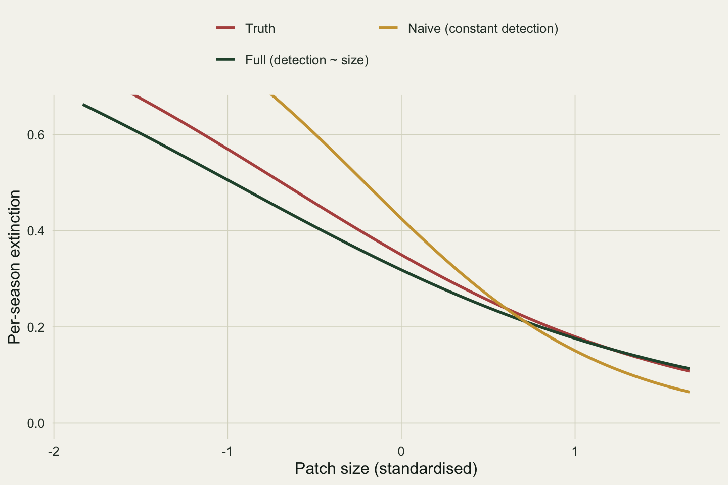
Colonisation survives more or less intact (naive slope 0.98 against the full model's 1.06). Extinction does not. The naive slope is -1.43, which is 1.83 times as steep as the full model's -0.78 and steeper than the truth of -0.9. Because detection genuinely rises with size, large patches produce more detections; a model with constant detection cannot say so, and instead explains the extra detections by making occupancy on large patches almost permanent. The size effect on extinction is inflated to absorb a detection signal that was never about extinction.
```{r}
#| label: fig-confound
#| fig-cap: "Per-season extinction against patch size from the correct model (detection modelled) and the naive one (detection held constant), with the truth. The naive curve falls too fast."
#| fig-alt: "Three extinction curves against patch size. Truth in red falls from about 0.74 to 0.11 and the full model in dark green from about 0.66 to 0.11. The naive curve in gold starts near 0.91 and falls to about 0.06, dropping more steeply than the other two."
#| fig-width: 7.5
#| fig-height: 5.0
ext_df <- bind_rows(
  data.frame(size = sg, val = plogis(e0 + e1 * sg),        model = "Truth"),
  data.frame(size = sg, val = plogis(pf[4] + pf[5] * sg), model = "Full (detection ~ size)"),
  data.frame(size = sg, val = plogis(pn[4] + pn[5] * sg), model = "Naive (constant detection)"))
ext_df$model <- factor(ext_df$model,
  levels = c("Truth", "Full (detection ~ size)", "Naive (constant detection)"))
ggplot(ext_df, aes(size, val, colour = model)) +
  geom_line(linewidth = 1) +
  scale_colour_manual(values = c("Truth" = "#b5534e",
    "Full (detection ~ size)" = "#275139", "Naive (constant detection)" = "#cda23f")) +
  coord_cartesian(ylim = c(0, 0.95)) +
  labs(x = "Patch size (standardised)", y = "Per-season extinction", colour = NULL) +
  theme_te() + guides(colour = guide_legend(nrow = 2))
```
Model selection sees through it. The detection covariate is real, and dropping it costs 187 AIC points (a likelihood-ratio statistic of 189 on one degree of freedom). The lesson is not that model comparison saves you, though it does here: it is that a covariate belongs on the detection rate whenever there is any reason to think detectability varies with it, because otherwise its effect reappears somewhere it does not belong.
## Where this leaves you
Covariates turn a description of average turnover into a statement about which sites are gaining and losing a species and why. The same design-matrix machinery extends to season effects (a covariate indexed by primary period rather than by site) and to survey-level detection covariates that change from visit to visit. With the rates in hand, the next question is what they imply for the occupancy trajectory and its equilibrium, which is [occupancy turnover and equilibrium](../occupancy-turnover-and-equilibrium/); and whether the fitted model actually fits, including whether detection is as homogeneous as assumed, is [checking a dynamic occupancy model](../checking-a-dynamic-occupancy-model/).
## References
- MacKenzie, Nichols, Hines, Knutson, Franklin 2003. Ecology 84(8):2200-2207 (10.1890/02-3090).
- Royle, Dorazio 2008. Hierarchical Modeling and Inference in Ecology. ISBN 978-0-12-374097-7.
- Kery, Royle 2021. Applied Hierarchical Modeling in Ecology, Volume 2. ISBN 978-0-12-809585-0.
- MacKenzie, Nichols, Royle, Pollock, Bailey, Hines 2018. Occupancy Estimation and Modeling, 2nd ed. ISBN 978-0-12-407197-1.
## Related tutorials
- [Dynamic occupancy: colonisation and extinction](../dynamic-occupancy-colonisation-extinction/)
- [Occupancy with detection covariates](../occupancy-detection-covariates/)
- [Occupancy turnover and equilibrium](../occupancy-turnover-and-equilibrium/)
- [Checking a dynamic occupancy model](../checking-a-dynamic-occupancy-model/)