---
title: "Occupancy turnover and equilibrium"
description: "Read the trajectory, equilibrium and turnover from a fitted dynamic occupancy model in base R, and see why a trend under constant rates need not mean change."
date: "2026-05-22 12:00"
categories: [occupancy, ecology tutorial, R, population dynamics]
image: thumbnail.png
image-alt: "Two occupancy trajectories under identical rates, one starting high and falling, one starting low and rising, both converging on a dashed equilibrium line."
---
Fitting a [dynamic occupancy model](../dynamic-occupancy-colonisation-extinction/) hands you colonisation, extinction and detection. Those rates are rarely the end of the analysis. What a manager wants is the occupancy this system is heading toward, how fast it moves, and how much of the occupied set is changing hands each season. All three follow from the two transition rates, and none of them require any new fitting: they are functions of the estimates you already have.
There is a reading error worth heading off first. If occupancy is falling season on season, the intuitive conclusion is that something is getting worse: extinction is rising, the habitat is degrading. That conclusion does not follow. A system with perfectly constant colonisation and extinction still shows a trend whenever it starts away from its equilibrium, and the trend can go either way. Reading the direction of change as a change in the rates is the mistake this tutorial is built to prevent.
## Fit a model and pull the rates
Three hundred sites, eight seasons, four visits. Occupancy starts high and the extinction rate exceeds colonisation, so the system is above its equilibrium.
```{r}
#| label: fit
set.seed(141)
R <- 300; Tn <- 8; K <- 4
psi1 <- 0.75; gamma <- 0.15; eps <- 0.25; p <- 0.40
z <- matrix(0L, R, Tn); z[, 1] <- rbinom(R, 1, psi1)
for (t in 2:Tn) z[, t] <- rbinom(R, 1, ifelse(z[, t - 1] == 1, 1 - eps, gamma))
d <- matrix(0L, R, Tn); for (t in 1:Tn) d[, t] <- rbinom(R, K, z[, t] * p)

emit <- function(dt, p, K) c(as.numeric(dt == 0), p^dt * (1 - p)^(K - dt))
site_ll <- function(dv, init, Phi, p, K) {
  a <- init * emit(dv[1], p, K); s <- sum(a); ll <- log(s); a <- a / s
  for (t in 2:length(dv)) {
    a <- as.vector(a %*% Phi) * emit(dv[t], p, K)
    s <- sum(a); ll <- ll + log(s); a <- a / s
  }
  ll
}
nll <- function(par, dat) {
  ps <- plogis(par[1]); ga <- plogis(par[2]); ep <- plogis(par[3]); pp <- plogis(par[4])
  Phi <- matrix(c(1 - ga, ga, ep, 1 - ep), 2, 2, byrow = TRUE)
  -sum(apply(dat, 1, site_ll, init = c(1 - ps, ps), Phi = Phi, p = pp, K = K))
}
fitfun <- function(dat) optim(c(0, qlogis(0.2), qlogis(0.2), qlogis(0.3)), nll,
                              dat = dat, method = "BFGS")
fit <- fitfun(d)
est <- plogis(fit$par); names(est) <- c("psi1", "gamma", "eps", "p")
round(est, 3)
```
The estimates are `psi1` 0.776, `gamma` 0.138, `eps` 0.241 and `p` 0.404, near the values that generated the data, with colonisation the loosest of the four.
## Equilibrium, trajectory, growth and turnover
The equilibrium occupancy is the level at which colonisation of empty sites exactly balances extinction of occupied ones: `psi* = gamma / (gamma + eps)`. The trajectory is the recursion `psi[t] = psi[t-1] (1 - eps) + (1 - psi[t-1]) gamma`, and the per-season growth ratio is one value of `psi[t+1] / psi[t]` for each interval.
```{r}
#| label: derived
psi_eq <- unname(est["gamma"] / (est["gamma"] + est["eps"]))
psit <- numeric(Tn); psit[1] <- est["psi1"]
for (t in 2:Tn) psit[t] <- psit[t - 1] * (1 - est["eps"]) + (1 - psit[t - 1]) * est["gamma"]
lambda <- psit[-1] / psit[-Tn]
turnover_eq <- (1 - psi_eq) * est["gamma"] / psi_eq   # colonised share of occupied at equilibrium
round(c(equilibrium = psi_eq, turnover = turnover_eq,
        growth_first = lambda[1], growth_last = lambda[Tn - 1]), 3)
```
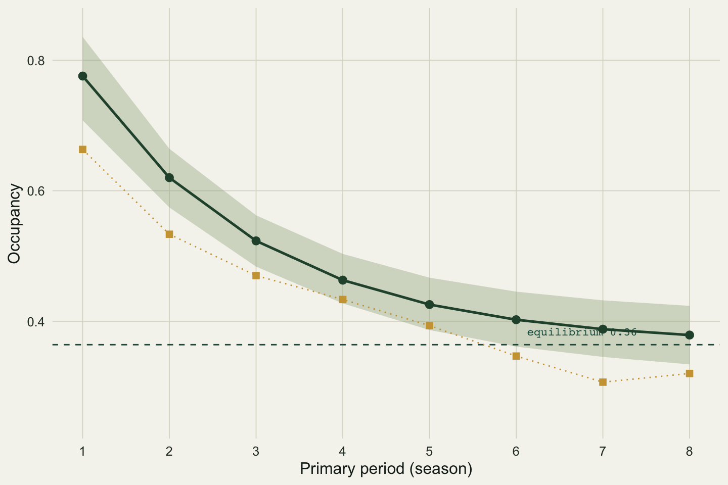
The equilibrium is 0.364. The trajectory starts at 0.776 and falls to 0.379 by season eight, sitting just above equilibrium. The growth ratio tells the same story from the side: it is 0.80 across the first interval (a 20 per cent drop) and climbs to 0.98 by the last, because the closer occupancy gets to equilibrium the less it moves. Turnover comes out at 0.241, and that is not a coincidence: at equilibrium the colonised fraction of the occupied set equals the extinction rate exactly. Roughly a quarter of the occupied sites in any season are freshly colonised, an equal number are lost, and the total holds steady even as individual sites change state.
```{r}
#| label: fig-trajectory-band
#| fig-cap: "Modelled occupancy trajectory with a parametric-bootstrap 95 per cent band, the estimated equilibrium (dashed), and the naive observed occupancy (gold squares) for reference."
#| fig-alt: "Occupancy against season. A dark green modelled curve falls from 0.78 to 0.38 inside a shaded band and levels near the dashed equilibrium at 0.36. Gold squares for naive observed occupancy track the same shape a little lower."
#| fig-width: 7.5
#| fig-height: 5.0
suppressMessages({library(ggplot2); library(dplyr)})
theme_te <- function(bs = 12) theme_minimal(base_size = bs) + theme(
  plot.background = element_rect(fill = "#f5f4ee", colour = NA),
  panel.background = element_rect(fill = "#f5f4ee", colour = NA),
  panel.grid.major = element_line(colour = "#dad9ca", linewidth = 0.3),
  panel.grid.minor = element_blank(),
  axis.text = element_text(colour = "#2c3a31"), axis.title = element_text(colour = "#16241d"),
  plot.title = element_text(colour = "#16241d", face = "bold"),
  plot.subtitle = element_text(colour = "#46604a"),
  legend.text = element_text(colour = "#2c3a31"), legend.position = "top",
  legend.key = element_rect(fill = "#f5f4ee", colour = NA))

simdat <- function(pr) {
  zz <- matrix(0L, R, Tn); zz[, 1] <- rbinom(R, 1, pr[1])
  for (t in 2:Tn) zz[, t] <- rbinom(R, 1, ifelse(zz[, t - 1] == 1, 1 - pr[3], pr[2]))
  dd <- matrix(0L, R, Tn); for (t in 1:Tn) dd[, t] <- rbinom(R, K, zz[, t] * pr[4]); dd
}
set.seed(1411); B <- 200; trb <- matrix(NA, B, Tn); eqb <- numeric(B)
for (b in 1:B) {
  fb <- plogis(fitfun(simdat(est))$par)
  eqb[b] <- fb[2] / (fb[2] + fb[3])
  tt <- numeric(Tn); tt[1] <- fb[1]
  for (t in 2:Tn) tt[t] <- tt[t - 1] * (1 - fb[3]) + (1 - tt[t - 1]) * fb[2]
  trb[b, ] <- tt
}
band <- data.frame(season = 1:Tn, lo = apply(trb, 2, quantile, 0.025),
                   hi = apply(trb, 2, quantile, 0.975))
df1 <- data.frame(season = 1:Tn, psit = psit, naive = colMeans(d > 0))
ggplot() +
  geom_ribbon(data = band, aes(season, ymin = lo, ymax = hi), fill = "#93a87f", alpha = 0.35) +
  geom_hline(yintercept = psi_eq, linetype = "dashed", colour = "#1d5b4e", linewidth = 0.5) +
  annotate("text", x = 2.5, y = psi_eq + 0.02, label = "equilibrium 0.36",
           colour = "#1d5b4e", size = 3, hjust = 1, family = "mono") +
  geom_line(data = df1, aes(season, psit), colour = "#275139", linewidth = 0.9) +
  geom_point(data = df1, aes(season, psit), colour = "#275139", size = 2.4) +
  geom_point(data = df1, aes(season, naive), colour = "#cda23f", shape = 15, size = 2.2) +
  geom_line(data = df1, aes(season, naive), colour = "#cda23f", linewidth = 0.5, linetype = "dotted") +
  scale_x_continuous(breaks = 1:Tn) + coord_cartesian(ylim = c(0.25, 0.85)) +
  labs(x = "Primary period (season)", y = "Occupancy") +
  theme_te()
```
## Uncertainty without a formula
The equilibrium is a ratio of two estimated rates, so a delta-method interval is possible, but a parametric bootstrap is easier to get right and reuses the fitting code. Simulate a fresh data set from the fitted parameters, refit, recompute the quantity, and repeat; the spread of the refits is the sampling distribution. The band in the figure above is exactly that, applied to the trajectory season by season.
```{r}
#| label: bootstrap-ci
round(c(equilibrium = psi_eq, lo = quantile(eqb, 0.025)[[1]], hi = quantile(eqb, 0.975)[[1]],
        season8 = psit[Tn], s8_lo = band$lo[Tn], s8_hi = band$hi[Tn]), 3)
```
The equilibrium is 0.364 with a 95 per cent interval of 0.318 to 0.412, and the season-eight occupancy carries a band of 0.334 to 0.424. The interval on a derived quantity is wider than a glance at the point estimate suggests, which is the reason to compute it rather than report a bare number.
## Same rates, opposite trends
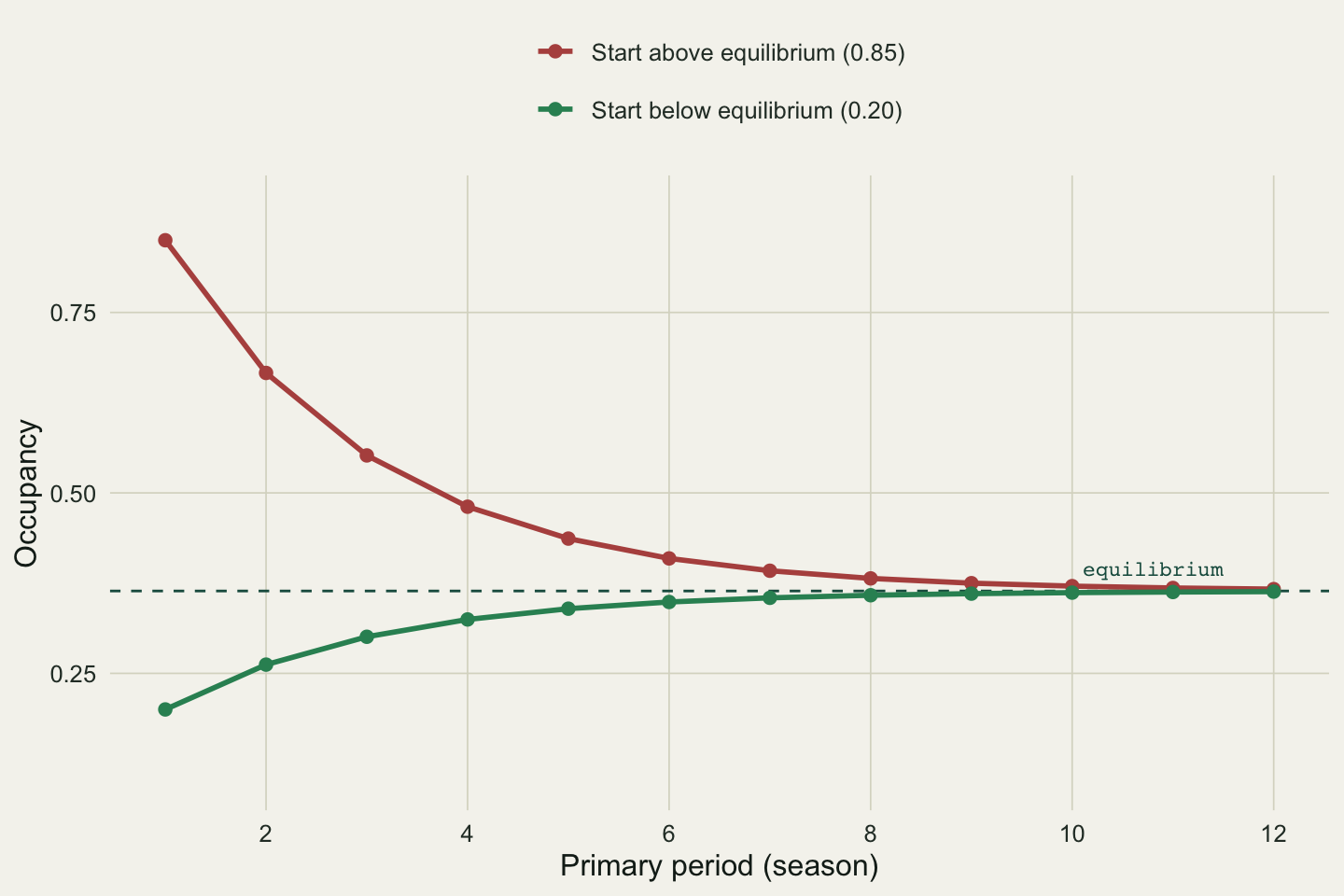
Here is the trap made concrete. Take the fitted colonisation and extinction and project two systems that differ only in where they start: one above equilibrium, one below. No stochasticity, no refitting, just the recursion.
```{r}
#| label: fig-transient
#| fig-cap: "Two projections under the same fitted colonisation and extinction, differing only in starting occupancy. Both converge on the same equilibrium from opposite directions."
#| fig-alt: "Two occupancy curves over twelve seasons. A red curve starts at 0.85 and falls, a green curve starts at 0.20 and rises, and both level off at the dashed equilibrium near 0.36."
#| fig-width: 7.5
#| fig-height: 5.0
proj <- function(p1, g, e, H) {
  v <- numeric(H); v[1] <- p1
  for (t in 2:H) v[t] <- v[t - 1] * (1 - e) + (1 - v[t - 1]) * g
  v
}
H <- 12
tr2 <- bind_rows(
  data.frame(season = 1:H, occ = proj(0.85, est["gamma"], est["eps"], H),
             start = "Start above equilibrium (0.85)"),
  data.frame(season = 1:H, occ = proj(0.20, est["gamma"], est["eps"], H),
             start = "Start below equilibrium (0.20)"))
ggplot(tr2, aes(season, occ, colour = start)) +
  geom_hline(yintercept = psi_eq, linetype = "dashed", colour = "#1d5b4e", linewidth = 0.5) +
  annotate("text", x = 11.5, y = psi_eq + 0.03, label = "equilibrium",
           colour = "#1d5b4e", size = 3, hjust = 1, family = "mono") +
  geom_line(linewidth = 1) + geom_point(size = 2) +
  scale_colour_manual(values = c("Start above equilibrium (0.85)" = "#b5534e",
    "Start below equilibrium (0.20)" = "#2f8f63")) +
  scale_x_continuous(breaks = seq(2, H, 2)) + coord_cartesian(ylim = c(0.1, 0.9)) +
  labs(x = "Primary period (season)", y = "Occupancy", colour = NULL) +
  theme_te() + guides(colour = guide_legend(nrow = 2))
```
The two systems have identical demographic rates. One declines, one recovers, and both settle at 0.364. A monitoring programme that saw only the first few seasons of the red line would report a worrying decline; one that saw the green line would report a recovery. Neither reading is about the rates, which never changed. The only way to separate a transient approach to equilibrium from a genuine change in colonisation or extinction is to estimate the rates, which is what the model does and a trend line does not.
## A note on the final season
One pair of quantities resists estimation. With season-specific rates, the colonisation and extinction over the last interval are confounded with each other. The four visits within the final season still pin down that season's detection probability, and through it the final occupancy, but occupancy in season `r Tn` is a single number reached from season `r Tn - 1` by two rates at once, and no later season exists to break them apart. Only their joint effect on that final occupancy is estimable. It is the same kind of wall the terminal parameters hit in [Cormack-Jolly-Seber survival](../cormack-jolly-seber-survival/), though there it is survival and detection that merge rather than two transition rates: the last few numbers of a time-varying model should be read with care or constrained, and the constant-rate model sidesteps the problem by borrowing strength across all intervals.
## References
- MacKenzie, Nichols, Hines, Knutson, Franklin 2003. Ecology 84(8):2200-2207 (10.1890/02-3090).
- Royle, Kery 2007. Ecology 88(7):1813-1823 (10.1890/06-0669.1).
- Kery, Royle 2021. Applied Hierarchical Modeling in Ecology, Volume 2. ISBN 978-0-12-809585-0.
- MacKenzie, Nichols, Royle, Pollock, Bailey, Hines 2018. Occupancy Estimation and Modeling, 2nd ed. ISBN 978-0-12-407197-1.
## Related tutorials
- [Dynamic occupancy: colonisation and extinction](../dynamic-occupancy-colonisation-extinction/)
- [Covariates in dynamic occupancy models](../dynamic-occupancy-covariates/)
- [Checking a dynamic occupancy model](../checking-a-dynamic-occupancy-model/)
- [Validating an SDM against a resurvey](../validating-an-sdm-against-a-resurvey/)