library(ggplot2)

te_paper  <- "#f5f4ee"
te_ink    <- "#16241d"
te_body   <- "#2c3a31"
te_forest <- "#275139"
te_rust   <- "#b5534e"
te_gold   <- "#c9b458"
te_line   <- "#dad9ca"

theme_datasheet <- function() {
  theme_minimal(base_size = 12) +
    theme(plot.background  = element_rect(fill = te_paper, colour = NA),
          panel.background = element_rect(fill = te_paper, colour = NA),
          panel.grid.major = element_line(colour = te_line, linewidth = 0.3),
          panel.grid.minor = element_blank(),
          text             = element_text(colour = te_body),
          plot.title       = element_text(colour = te_ink, face = "bold"),
          plot.subtitle    = element_text(colour = te_body),
          axis.text        = element_text(colour = te_body),
          strip.text       = element_text(colour = te_ink))
}Classifier scores over a camera-trap sequence
R
camera traps
model evaluation
machine learning
simulation
ecology tutorial
Averaging calibrated per-image scores over a camera-trap burst: a closed form for the calibration slope, what empty frames do to it, and recalibration in R.
A camera trap fires and writes a burst of five photographs. An image classifier scores each photograph separately and returns a probability that a pine marten is in it, and the classifier has been calibrated on labelled images, so that of all images scored 0.3 about three in ten really do hold a marten. The survey, however, needs one answer per burst: was there a marten in front of the camera or not. So the five numbers are combined, by averaging them, by taking the largest, or by treating the five images as five independent pieces of evidence and combining their odds, and the combined number is read as the probability that the sequence holds the animal.
None of the three combinations is calibrated just because the images are. Five photographs taken within a second or two share the same light, the same background, the same wet grass moving in the same wind, so the errors of the classifier are correlated within the burst. And a positive burst does not show the animal in every frame: a marten that crosses the edge of the field of view is in two photographs and absent from three. The first problem makes an averaged score too timid or a multiplied one too bold by an amount that can be written down. The second pulls every rule towards overconfidence, and most of them towards too low an average, by amounts that depend on how often the animal is actually in frame, which the image-level calibration cannot tell apart from how often it passes the camera.
The single-probability version of this problem is covered in Calibrating predicted probabilities in R, which builds reliability diagrams and fits Platt scaling to one probability per plot; its section on what calibration cannot tell you is about moving a calibrated model to a new population. The move here is a different one: from the unit the classifier was calibrated on, the image, to the unit the survey needs, the sequence. Score thresholds and precision in bioacoustics and Automated acoustic detections as data work with one score per clip and a threshold on it; nothing there pools several scores for one event. The closest relative is Two imperfect tests and no gold standard, whose section on dependence the fit cannot see shows what conditionally dependent tests do to a latent class model; five frames of one burst are five conditionally dependent tests, pooled rather than used to estimate accuracies. And Checking a camera trap density estimate makes the counting side of the same point: a burst of photographs of one deer is one crossing seen several times.
The post first derives the calibration slope of the averaged and the multiplied score when every frame of a positive burst shows the animal, and checks the formula against simulation; that part is arithmetic and is presented as such. The measured content is what follows: what frames without the animal do to five combination rules, and how many labelled sequences a sequence-level recalibration needs.
When the animal is in every frame, the slope is a closed form
Take the mean logit first. Each calibrated frame logit is a linear function of the raw score, L = c + b z with b = 2 / 2.25, so the mean logit is c + b times the mean raw score. Within a sequence the mean raw score keeps the variance of the shared noise in full and the variance of the frame noise divided by five, so its variance is 2.25 v with v = s + (1 - s) / m. The frame calibration was built for a single frame, whose variance is 2.25; the mean has variance 2.25 v, and with two normal classes of equal variance the true sequence log-odds is linear in the mean score with slope 2 / (2.25 v) = b / v. The calibration slope of the mean logit is therefore exactly 1 / v, or
k = 1 / (s + (1 - s) / m).
The independence product is m times the mean logit minus a constant, so its slope is k / m. At s = 0 the mean logit is too timid by a factor of m and the product is exactly right, which is the case naive Bayes is built for; at s = 1 the five frames are one frame five times, the mean is exactly right, and the product is m times too bold. Everything between is the formula. This is standard algebra for averaging correlated normal scores and is not a finding of this post; the chunk below reproduces it and adds the three rules that have no such formula.
s_grid <- seq(0.1, 0.9, by = 0.1)
set.seed(43902)
cf_tab <- do.call(rbind, lapply(s_grid, run_cell, p_f = 1))
cf_tab$v_sh   <- cf_tab$s_sh + (1 - cf_tab$s_sh) / m_fr
cf_tab$closed <- ifelse(cf_tab$rule == "mean_logit", 1 / cf_tab$v_sh,
                  ifelse(cf_tab$rule == "product", 1 / (m_fr * cf_tab$v_sh), NA))
cf_chk  <- cf_tab[!is.na(cf_tab$closed), ]
cf_z    <- (cf_chk$slope - cf_chk$closed) / cf_chk$se
cf_rel  <- abs(cf_chk$slope / cf_chk$closed - 1)
cf_get  <- function(s_v, r) cf_tab$slope[abs(cf_tab$s_sh - s_v) < 1e-9 & cf_tab$rule == r]
cf_se_max <- max(cf_tab$se)
nor_tab   <- cf_tab[cf_tab$rule == "noisy_or", ]
stopifnot(all(diff(nor_tab$slope) < 0))
nor_cross <- approx(nor_tab$slope, nor_tab$s_sh, xout = 1)$y
Over 9 values of s from 0.1 to 0.9, each with 50000 held-out sequences, the simulated slopes of the mean logit and the product differ from the formula by at most 1.1 per cent and at most 1.1 standard errors of the fitted slope; the largest standard error of any slope in the table is 0.042. At s = 0.1 the formula gives 3.571 for the mean logit and the simulation 3.567; at s = 0.5 it gives 1.667 against 1.677; at s = 0.9, 1.087 against 1.092. The product at the same three values is 0.713, 0.335 and 0.218, against 0.714, 0.333 and 0.217.
The three rules without a formula behave differently from each other. The mean probability is more timid than the mean logit at s = 0.1, 4.328. The largest probability runs from 1.941 at s = 0.1 to 1.066 at s = 0.9. The noisy-OR crosses one: 1.643 at s = 0.1 and 0.504 at s = 0.9. With the animal in every frame no rule is calibrated at every s, and which one comes closest depends on s.
cf_plot <- cf_tab
cf_plot$rule <- factor(rule_lab[cf_plot$rule], rule_lab)
s_fine  <- seq(0.05, 0.95, by = 0.01)
cf_line <- rbind(
  data.frame(s_sh = s_fine, slope = 1 / (s_fine + (1 - s_fine) / m_fr), rule = rule_lab[["mean_logit"]]),
  data.frame(s_sh = s_fine, slope = 1 / (m_fr * (s_fine + (1 - s_fine) / m_fr)), rule = rule_lab[["product"]]))
cf_line$rule <- factor(cf_line$rule, rule_lab)
rule_cols <- c(te_gold, te_forest, te_ink, te_body, te_rust)
rule_shapes <- c(17, 16, 15, 5, 16)
names(rule_cols) <- names(rule_shapes) <- rule_lab

ggplot(cf_plot, aes(s_sh, slope, colour = rule)) +
  geom_hline(yintercept = 1, linetype = "dashed", colour = te_body, linewidth = 0.5) +
  geom_line(data = cf_line, linewidth = 0.9, show.legend = FALSE) +
  geom_point(aes(shape = rule), size = 2.4) +
  scale_y_log10(breaks = c(0.2, 0.3, 0.5, 1, 2, 3, 5)) +
  scale_colour_manual(values = rule_cols, breaks = rule_lab, name = NULL) +
  scale_shape_manual(values = rule_shapes, breaks = rule_lab, name = NULL) +
  labs(x = "share of the noise shared within a sequence, s",
       y = "calibration slope (log scale)",
       title = "Averaging correlated scores has a known slope",
       subtitle = "above 1: too timid; below 1: too extreme; lines: 1/v and 1/(m v)") +
  theme_datasheet() +
  theme(legend.position = "bottom") +
  guides(colour = guide_legend(nrow = 2, byrow = TRUE), shape = guide_legend(nrow = 2, byrow = TRUE))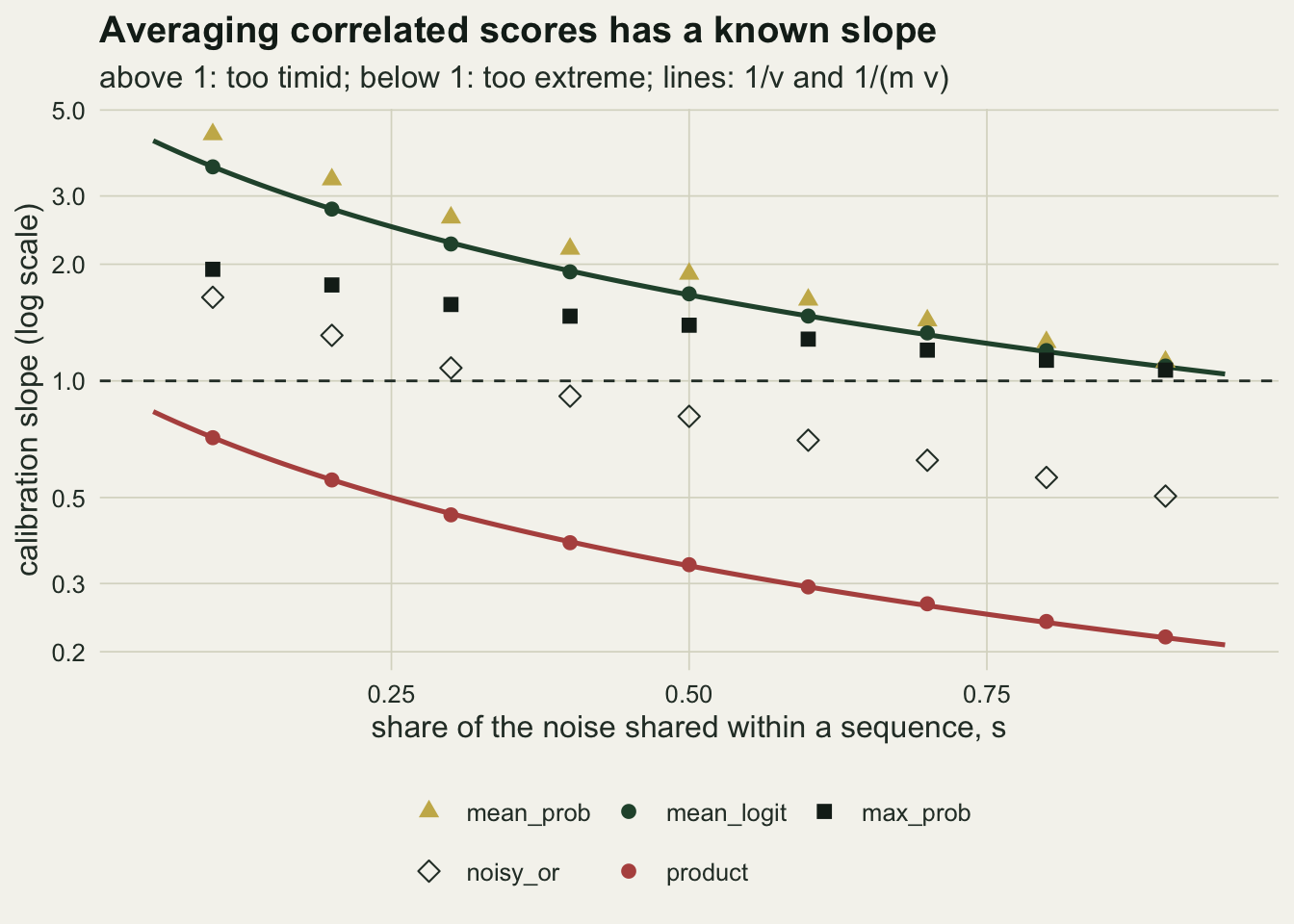
Frames without the animal turn the rules overconfident
Now let the animal be absent from some frames of a positive sequence. The slope of the frame calibration is unchanged, because frame by frame the two classes are still the same two normals; its intercept follows the lower frame prevalence, 0.3 pf, so every frame stays perfectly calibrated. What changes is the mean raw score of a positive sequence: it is now 2 times the share of frames with the animal, which averages pf rather than one. A first-order version of the argument above, which ignores the extra spread from the number of occupied frames varying between sequences, says the true sequence log-odds rises with the mean score at pf times the old rate while the mean logit rises at the same rate as before. So the slope of the mean logit is roughly pf / v: the shared noise pushes it above one by a factor 1 / v, the empty frames pull it below by a factor pf, and it crosses one where pf is near v. That approximation is only a guide; the simulation below measures the slope over a grid of pf for three values of s.
pf_grid <- seq(1, 0.2, by = -0.1)
s_three <- c(0.1, 0.5, 0.9)
set.seed(43903)
pf_tab <- do.call(rbind, lapply(s_three, function(s_v)
  do.call(rbind, lapply(pf_grid, function(p_v) run_cell(s_v, p_v)))))
pf_tab$v_sh   <- pf_tab$s_sh + (1 - pf_tab$s_sh) / m_fr
pf_tab$approx <- pf_tab$p_f / pf_tab$v_sh
pf_get <- function(s_v, p_v, r, col = "slope") pf_tab[[col]][abs(pf_tab$s_sh - s_v) < 1e-9 &
                                             abs(pf_tab$p_f - p_v) < 1e-9 & pf_tab$rule == r]

ml_tab   <- pf_tab[pf_tab$rule == "mean_logit", ]
ml_ratio <- ml_tab$slope / ml_tab$approx
cross_pf <- sapply(s_three, function(s_v) {
  d_s <- ml_tab[abs(ml_tab$s_sh - s_v) < 1e-9, ]
  if (all(d_s$slope > 1)) NA else approx(d_s$slope, d_s$p_f, xout = 1)$y
})
stopifnot(sum(ml_ratio[ml_tab$p_f < 1] < 1) == sum(ml_tab$p_f < 1))
n_ml_2se <- sum(((ml_tab$approx - ml_tab$slope) / ml_tab$se)[ml_tab$p_f < 1] > 2)
mp_tab   <- pf_tab[pf_tab$rule == "mean_prob", ]
stopifnot(max(abs(mp_tab$mean_pred - prev * mp_tab$p_f)) < 0.005)
within10 <- tapply(abs(pf_tab$slope - 1) <= 0.1, pf_tab$rule, sum)
n_cells  <- length(s_three) * length(pf_grid)
se_pf_max <- max(pf_tab$se)
At s = 0.5 the mean logit goes from 1.687 with the animal in every frame to 0.934 at pf = 0.6, 0.614 at pf = 0.4 and 0.495 at pf = 0.3: from too timid to too extreme. At s = 0.9 it is already below one at pf = 0.9, 0.964, and reaches 0.320 at pf = 0.3. At s = 0.1 the pull of the correlation is the stronger one down to pf = 0.4, where the slope is 1.308; it is 1.885 at pf = 0.6, 0.969 at pf = 0.3 and 0.670 at pf = 0.2. By linear interpolation the mean logit crosses a slope of one at pf = 0.31, 0.64 and 0.93 for s = 0.1, 0.5 and 0.9, where v is 0.28, 0.60 and 0.92. The rough approximation pf / v is within 12 per cent of the simulated slope over the whole grid and above it in every one of the 24 cells with pf < 1 (at pf = 1 it is the exact closed form), by more than two standard errors of the fitted slope in 17 of them; the largest standard error of any slope here is 0.041.
The other rules move the same way. The largest probability, 1.914 at s = 0.1 with the animal in every frame, is 0.806 at pf = 0.3; at s = 0.5 it goes from 1.396 to 0.675. The noisy-OR, which was already below one at s = 0.5, goes from 0.810 to 0.531. The independence product is below one everywhere on the grid and reaches 0.043. Over the 27 combinations of s and pf, the mean probability has a slope within ten per cent of one in 3, the mean logit in 4, the largest probability in 8, the noisy-OR in 1 and the independence product in 0. For the mean probability, the mean logit and the largest probability the two forces pull in opposite directions, and each of them is calibrated only where they happen to cancel. For the independence product at every s, and for the noisy-OR once s is above 0.35 (where its slope with the animal in every frame crosses one), both push towards overconfidence. The image-level calibration shows neither force: it is the same for every s, and it sees pf only through the frame prevalence 0.3 pf.
em_plot <- pf_tab[pf_tab$rule %in% c("mean_logit", "max_prob"), ]
em_plot$rule  <- factor(rule_lab[em_plot$rule], rule_lab[c("mean_logit", "max_prob")])
em_plot$s_lab <- factor(sprintf("s = %.1f", em_plot$s_sh))
em_appr <- ml_tab
em_appr$rule  <- factor(rule_lab[["mean_logit"]], rule_lab[c("mean_logit", "max_prob")])
em_appr$s_lab <- factor(sprintf("s = %.1f", em_appr$s_sh))

ggplot(em_plot, aes(p_f, slope, colour = s_lab)) +
  geom_hline(yintercept = 1, colour = te_body, linewidth = 0.5) +
  geom_line(data = em_appr, aes(y = approx), linetype = "dashed", linewidth = 0.6) +
  geom_line(linewidth = 0.9) +
  geom_point(size = 2) +
  facet_wrap(~ rule) +
  scale_y_log10(breaks = c(0.3, 0.5, 0.7, 1, 1.5, 2, 3)) +
  scale_x_reverse(breaks = seq(1, 0.2, by = -0.2)) +
  scale_colour_manual(values = c(te_forest, te_gold, te_rust), name = NULL) +
  labs(x = "probability that a frame of a positive sequence shows the animal, pf",
       y = "calibration slope (log scale)",
       title = "Empty frames pull the slope down",
       subtitle = "solid: simulated; dashed: pf / v for the mean logit") +
  theme_datasheet() +
  theme(legend.position = "bottom")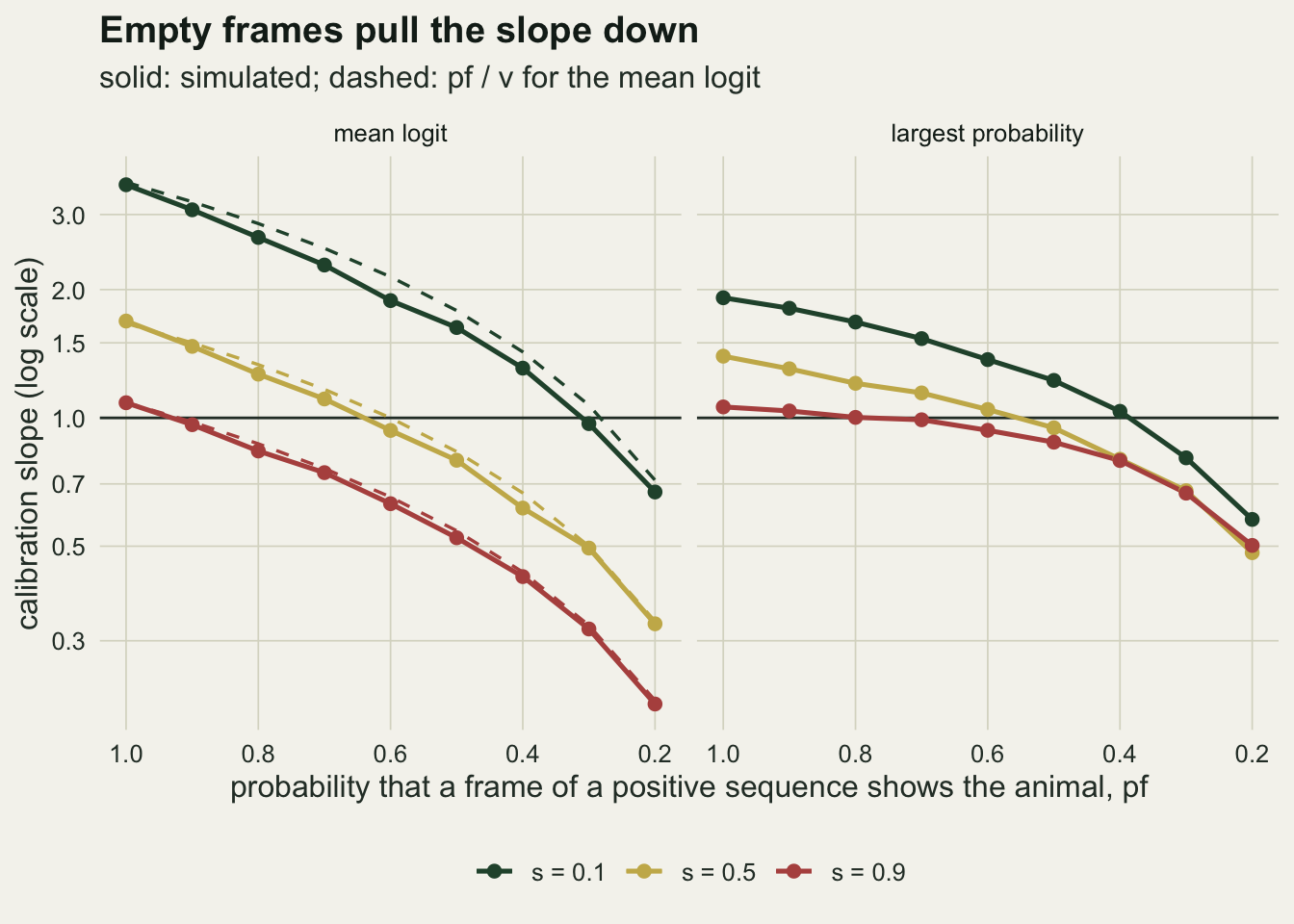
The slope is not the only thing that goes wrong. The mean probability averages exactly the frame prevalence, 0.3 pf, because each calibrated frame probability does, and with empty frames that is lower than the sequence prevalence; the other rules have no such anchor and miss on either side. At s = 0.5 and pf = 0.3 the held-out sequences hold the animal in 0.303 of cases, while the average prediction is 0.071 for the mean logit, 0.090 for the mean probability, 0.195 for the largest probability, 0.341 for the noisy-OR and 0.148 for the independence product. With the animal in every frame the same five averages are 0.286, 0.300, 0.476, 0.715 and 0.340 against 0.300. The average error (calibration in the large) and the slope are different quantities: with the animal in every frame the mean probability has the right average and a slope of 1.903, so both need reporting.
A reliability diagram drawn on the logit scale shows the two at once. For s = 0.5 the held-out sequences are cut into ten equal-count bins of the mean-logit prediction, and the observed share of positive sequences in each bin is set against the mean prediction in the bin, both as logits.
rel_one <- function(p_f) {
  te <- gen_seq(n_test, 0.5, p_f)
  p_seq <- plogis(rowMeans(frame_logit(te$z, p_f)))
  bin_id <- cut(rank(p_seq, ties.method = "first"), 10, labels = FALSE)
  data.frame(p_f, pred = tapply(p_seq, bin_id, mean), obs = tapply(te$y, bin_id, mean))
}
set.seed(43904)
rel_tab <- rbind(rel_one(1), rel_one(0.3))
rel_span <- sapply(c(1, 0.3), function(p_v) {
  d_r <- rel_tab[rel_tab$p_f == p_v, ]
  diff(range(qlogis(d_r$obs))) / diff(range(qlogis(d_r$pred)))
})
rel_hi  <- rel_tab[rel_tab$p_f == 0.3, ][10, ]
rel_lo  <- rel_tab[rel_tab$p_f == 0.3, ][1, ]
rel_top <- rel_tab[rel_tab$p_f == 1, ][10, ]
stopifnot(all(rel_tab$obs[rel_tab$p_f == 0.3] > rel_tab$pred[rel_tab$p_f == 0.3]))
With the animal in every frame the top bin predicts 0.753 and 0.908 of its sequences are positive, and from the lowest bin to the highest the observed logit covers 1.62 times the range of the predicted one: the rule understates how sure it can be. With pf = 0.3 every bin lies above the diagonal, from 0.008 predicted against 0.161 observed in the lowest bin to 0.254 against 0.553 in the highest, and the observed logit covers only 0.50 times the predicted range: too low on average and too spread out. Each frame is perfectly calibrated in both; only what happens between the frames has changed.
rel_tab$panel <- factor(ifelse(rel_tab$p_f == 1, "animal in every frame", "animal in 30 per cent of frames"),
                        c("animal in every frame", "animal in 30 per cent of frames"))
p_brk <- c(0.01, 0.03, 0.1, 0.3, 0.5, 0.7, 0.9)
ggplot(rel_tab, aes(qlogis(pred), qlogis(obs), colour = panel)) +
  geom_abline(slope = 1, intercept = 0, linetype = "dashed", colour = te_body, linewidth = 0.5) +
  geom_line(linewidth = 0.9) +
  geom_point(size = 2.4) +
  scale_x_continuous(breaks = qlogis(p_brk), labels = p_brk) +
  scale_y_continuous(breaks = qlogis(p_brk), labels = p_brk) +
  scale_colour_manual(values = c(te_forest, te_rust), name = NULL) +
  coord_equal(xlim = qlogis(c(0.005, 0.95)), ylim = qlogis(c(0.005, 0.95))) +
  labs(x = "mean predicted probability in the bin (logit scale)",
       y = "observed share positive (logit scale)",
       title = "Same frames, two different failures",
       subtitle = "mean logit of five calibrated frames, s = 0.5") +
  theme_datasheet() +
  theme(legend.position = "bottom")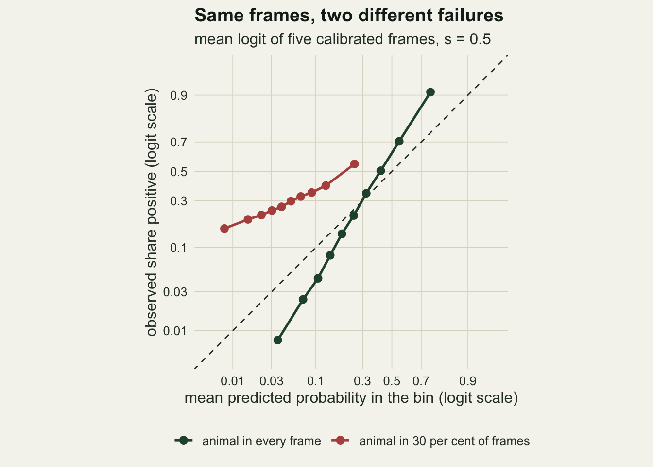
Recalibrating on labelled sequences, and how many it takes
The repair is to calibrate at the unit the survey uses. Take a set of sequences whose labels were checked by eye, compute the mean logit of each, and fit Platt scaling of the sequence label on it. The recalibrated prediction is then scored on the held-out sequences, which play no part in the fit.
There is a shortcut that makes the sweep cheap. The recalibrated logit is a + b times the mean logit, and a logistic regression of the held-out labels on a + b x has slope equal to the slope on x divided by b, because maximum likelihood does not care how the covariate is shifted and scaled. So the held-out calibration slope after recalibration is k_test / b, where k_test is the held-out slope of the uncorrected mean logit, fitted once. The chunk checks the identity on one recalibration fit by refitting directly, then draws 1000 fresh calibration sets at each of four sizes for two cases at s = 0.5, one timid (pf = 1) and one overconfident (pf = 0.3).
n_cal_set <- c(100, 300, 1000, 3000)
n_rep     <- 1000
set.seed(43905)
recal_rows <- list()
id_gap <- numeric(0)
k_rel  <- numeric(0)
for (p_f in c(1, 0.3)) {
  te <- gen_seq(n_test, 0.5, p_f)
  ml_te  <- rowMeans(frame_logit(te$z, p_f))
  k_fit  <- fit_slope(ml_te, te$y)
  k_rel  <- c(k_rel, k_fit[["se"]] / k_fit[["slope"]])
  cal_one <- gen_seq(300, 0.5, p_f)
  rc_one  <- fit_slope(rowMeans(frame_logit(cal_one$z, p_f)), cal_one$y)
  direct  <- fit_slope(rc_one[["int"]] + rc_one[["slope"]] * ml_te, te$y)[["slope"]]
  id_gap  <- c(id_gap, abs(direct - k_fit[["slope"]] / rc_one[["slope"]]))
  for (n_cal in n_cal_set) {
    b_hat <- replicate(n_rep, {
      cal <- gen_seq(n_cal, 0.5, p_f)
      fit_slope(rowMeans(frame_logit(cal$z, p_f)), cal$y)[["slope"]]
    })
    held <- k_fit[["slope"]] / b_hat
    se_n <- k_fit[["se"]] * sqrt(n_test / n_cal)
    pred_in <- pnorm(k_fit[["slope"]] / 0.9, k_fit[["slope"]], se_n) -
      pnorm(k_fit[["slope"]] / 1.1, k_fit[["slope"]], se_n)
    recal_rows[[length(recal_rows) + 1]] <- data.frame(p_f, n_cal, k_test = k_fit[["slope"]],
      q05 = unname(quantile(held, 0.05)), q50 = median(held), q95 = unname(quantile(held, 0.95)),
      in10 = mean(abs(held - 1) <= 0.1), pred_in = pred_in)
  }
}
stopifnot(max(id_gap) < 1e-6)
recal_tab <- do.call(rbind, recal_rows)
recal_tab$in10_se <- sqrt(recal_tab$in10 * (1 - recal_tab$in10) / n_rep)
rv <- function(p_v, n_v, col) recal_tab[recal_tab$p_f == p_v & recal_tab$n_cal == n_v, col]
in10_se_max <- max(recal_tab$in10_se)
pred_gap    <- max(abs(recal_tab$in10 - recal_tab$pred_in))
print(format(recal_tab, digits = 3), row.names = FALSE)
p_f n_cal k_test q05 q50 q95 in10 pred_in in10_se
1.0 100 1.652 0.681 0.968 1.39 0.361 0.374 0.01519
1.0 300 1.652 0.804 0.984 1.19 0.595 0.601 0.01552
1.0 1000 1.652 0.874 0.989 1.11 0.841 0.873 0.01156
1.0 3000 1.652 0.931 0.993 1.06 0.991 0.990 0.00299
0.3 100 0.473 0.496 0.961 3.16 0.173 0.174 0.01196
0.3 300 0.473 0.671 1.002 1.78 0.282 0.297 0.01423
0.3 1000 0.473 0.790 0.983 1.30 0.500 0.513 0.01581
0.3 3000 0.473 0.864 0.989 1.13 0.762 0.769 0.01347The identity holds to rounding error on the direct refits (the chunk checks that the difference is below 0.000001). With the animal in every frame, a recalibration on 100 labelled sequences gives a held-out slope between 0.68 and 1.39 (5th to 95th percentile over the 1000 calibration sets) and lands within ten per cent of one in 36 per cent of them; at 300 sequences, 0.80 to 1.19 and 60 per cent; at 1000, 0.87 to 1.11 and 84 per cent. With pf = 0.3 the same sizes give 0.50 to 3.16 (17 per cent within ten per cent), 0.67 to 1.78 (28 per cent) and 0.79 to 1.30 (50 per cent), and it takes 3000 sequences to reach 76 per cent. The Monte Carlo standard error of any of these shares is at most 0.016. The medians sit between 0.96 and 1.00, a little below one at the smallest sizes: the recalibration is close to unbiased, and the problem is its spread.
That spread is the ordinary sampling error of a logistic slope, and it can be predicted from the standard error of the slope in the large held-out fit scaled to the calibration size, treating the fitted slope as normal. That prediction of the share within ten per cent differs from the simulated share by at most 0.032 across the eight cells, so the sweep adds a size in sequences, not a new mechanism. What it does show is how much the empty frames cost in labels. The relative standard error of the slope, per labelled sequence, is 2.22 times larger with pf = 0.3 than with the animal in every frame, because the mean logit separates positive from empty sequences less well, and the number of sequences needed for the same precision grows with its square, 4.9 times. The size of a recalibration set is the size of a validation set for the calibration slope, the question Riley and colleagues (2021) answer for clinical prediction models, and the same calculation applies here.
recal_tab$case <- factor(ifelse(recal_tab$p_f == 1, "animal in every frame", "animal in 30 per cent of frames"),
                         c("animal in every frame", "animal in 30 per cent of frames"))
ggplot(recal_tab, aes(n_cal, q50, colour = case)) +
  annotate("rect", xmin = 70, xmax = 4300, ymin = 0.9, ymax = 1.1, fill = te_line, alpha = 0.6) +
  geom_hline(yintercept = 1, colour = te_body, linewidth = 0.5) +
  geom_errorbar(aes(ymin = q05, ymax = q95), width = 0.08, linewidth = 0.8,
                position = position_dodge(width = 0.15)) +
  geom_point(size = 2.6, position = position_dodge(width = 0.15)) +
  scale_x_log10(breaks = n_cal_set) +
  scale_y_log10(breaks = c(0.5, 0.7, 0.9, 1, 1.1, 1.5, 2, 3)) +
  scale_colour_manual(values = c(te_forest, te_rust), name = NULL) +
  labs(x = "labelled sequences in the recalibration set (log scale)",
       y = "held-out calibration slope (log scale)",
       title = "Recalibration works, given enough sequences",
       subtitle = "5th to 95th percentile over 1000 calibration sets") +
  theme_datasheet() +
  theme(legend.position = "bottom")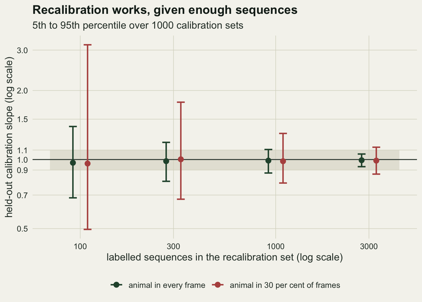
What to report
Say which unit the classifier was calibrated on and which unit the analysis uses. A statement that the classifier is calibrated means the image; if the occupancy model or the activity index is built from sequences, the calibration of the sequence rule is a separate claim and has to be checked on sequences.
Report the rule used to combine frames, and its calibration slope and its calibration in the large on held-out labelled sequences, with the number of sequences. Calibration in the large is the average prediction against the observed rate, or on the logit scale the intercept of the calibration model with the slope fixed at one (Van Calster et al. 2019). None of the five rules above is calibrated in general, and the direction of its error depends on two quantities of the deployment: how correlated the classifier’s errors are within a burst, and how often the animal is actually in frame.
The first of those can be estimated from sequences checked as empty, where every frame’s score is noise. A one-way analysis of variance of the calibrated frame logits, with sequence as the group, gives the intraclass correlation.
set.seed(43906)
icc_est <- sapply(c(0.1, 0.5, 0.9), function(s_v) {
  cal <- gen_seq(300, s_v, 1)
  z_neg <- cal$z[cal$y == 0, ]
  n_g   <- nrow(z_neg)
  ms_b  <- m_fr * sum((rowMeans(z_neg) - mean(z_neg))^2) / (n_g - 1)
  ms_w  <- sum((z_neg - rowMeans(z_neg))^2) / (n_g * (m_fr - 1))
  c(n_neg = n_g, icc = (ms_b - ms_w) / (ms_b + (m_fr - 1) * ms_w))
})
In one calibration set of 300 sequences for each value, the 203, 216 and 214 empty ones give intraclass correlations of 0.12, 0.48 and 0.88 for true shares of 0.1, 0.5 and 0.9. Raw scores and calibrated logits give the same value, since one is a linear function of the other. Report it: with the share of frames showing the animal in positive sequences, it places a deployment on the pf / v map above and, away from the crossing, says in which direction the uncorrected mean logit will be wrong. It does not replace the sequence-level recalibration, which fixes both at once.
Budget the labelled sequences before labelling. In this setting 300 sequences brought the slope within ten per cent of one in 60 per cent of calibration sets when the animal is in every frame, and 1000 did so in 50 per cent when it is in 30 per cent of frames. The normal approximation above predicted these shares from the standard error of a single large fit, so the budget is an ordinary sample-size calculation for a logistic slope rather than something that needs simulating.
Honest limits
The raw scores are normal with equal variance in both classes, which makes the frame-level Platt fit exact and the closed form exact. Real classifier logits are not normal: deep networks produce scores piled against zero and one, with long tails, and a Platt fit to them is an approximation. The closed form then holds only roughly, and a reliability diagram of the frame calibration is the first thing to look at.
The within-sequence dependence is a single shared random intercept with the same s for positive and negative sequences. In real bursts the dependence also runs through the signal: the same animal in the same pose is scored alike in every frame, and a positive sequence may be more or less correlated than an empty one. Nothing here separates those.
Frames show the animal independently with probability pf. A real animal enters, stays and leaves, so its frames come in a run, and the number of occupied frames varies between sequences in a way the binomial does not describe. The direction of the effect should survive that; its size was not measured.
Every sequence has five frames and the prevalence is fixed at 0.3. With bursts of different lengths the mean logit of a long burst and a short one have different variances, so one recalibration line for all of them is itself miscalibrated; fitting the recalibration with the burst length as a covariate is the obvious extension and was not tried.
Only the calibration slope was studied, and only calibration. A rule can be well calibrated after recalibration and still rank sequences worse than another rule would; whether the largest probability or the mean logit separates positive from empty sequences better at low pf is a discrimination question this post does not answer. The recalibration used the mean logit alone; a logistic model on two summaries, such as the mean and the largest logit, may do better and was not measured.
The sequence labels used to recalibrate are treated as correct. Labels checked by eye miss animals at the edge of the frame, which is exactly the low-pf case, and label error in the recalibration set is not modelled.
References
Cox DR 1958 Biometrika 45(3-4):562-565 (10.1093/biomet/45.3-4.562)
Van Calster B, McLernon DJ, van Smeden M, Wynants L, Steyerberg EW 2019 BMC Medicine 17(1):230 (10.1186/s12916-019-1466-7)
Hand DJ, Yu K 2001 International Statistical Review 69(3):385-398 (10.1111/j.1751-5823.2001.tb00465.x)
Niculescu-Mizil A, Caruana R 2005 Proceedings of the 22nd International Conference on Machine Learning:625-632 (10.1145/1102351.1102430)
Riley RD, Debray TPA, Collins GS, Archer L, Ensor J, van Smeden M, Snell KIE 2021 Statistics in Medicine 40(19):4230-4251 (10.1002/sim.9025)