library(ggplot2)

te_pal <- list(forest = "#275139", green = "#2f8f63", sage = "#93a87f",
               clay = "#b5534e", gold = "#cda23f", line = "#dad9ca",
               ink = "#16241d", paper = "#f5f4ee")

theme_te <- function() {
  theme_minimal(base_size = 12) +
    theme(panel.grid.minor = element_blank(),
          panel.grid.major = element_line(colour = "#e7e6dc"),
          plot.background = element_rect(fill = "#f5f4ee", colour = NA),
          panel.background = element_rect(fill = "#f5f4ee", colour = NA),
          plot.title = element_text(face = "bold", colour = te_pal$ink),
          axis.title = element_text(colour = "#2c3a31"))
}Estimating R0 from incidence data
R
epidemiology
disease ecology
GLM
ecology tutorial
ggplot2
Estimate the reproduction number from an epidemic curve in R: Poisson growth rates by hand, the generation interval map, and a renewal equation Rt estimate.
A wildlife disease outbreak arrives as a column of numbers: cases found per day, or per week, in a sampled population. The quantity everyone wants from that column is the basic reproduction number, the average number of secondary infections one infectious individual produces in a fully susceptible population, because it sets the threshold for control. Above one the outbreak grows, below one it dies out, and the fraction of the population that has to be immunised or removed to push it below one is \(1 - 1/R_0\).
The column of numbers does not contain \(R_0\). It contains a growth rate. Getting from one to the other requires a second ingredient, the generation interval distribution, which describes the time between one individual becoming infected and the individuals it infects becoming infected. That distribution is almost never measured in a wildlife system, so it is assumed, and the assumption sets the answer. This post measures how much.
Two estimators are coded by hand here. The first fits an exponential growth rate to the early part of the curve by Poisson regression and maps it through the generation interval to a single \(R_0\). The second drops the exponential assumption entirely and estimates a reproduction number for every day using the renewal equation, which is what you need when control measures come in partway through and the number is moving. The SEIR model and the latent period is where the map from growth rate to reproduction number comes from, and it is worth reading first: the algebra below is that model’s Euler-Lotka equation, rearranged so the growth rate is the input rather than the output.
A simulated outbreak with a known reproduction number
The simulator is a discrete time renewal process with susceptible depletion. On day \(t\) the force of infection is the weighted sum of past incidence, \(\Lambda_t = \sum_s w_s I_{t-s}\), where \(w\) is the generation interval distribution discretised to whole days, and new cases are Poisson with mean \(R_t \, (S_t / N) \, \Lambda_t\). Susceptibles are then decremented by the cases. This is the same bookkeeping as a stochastic SEIR model, written in a form that makes the generation interval explicit rather than implied by the transition rates, which matters here because the generation interval is the object under test.
Everything is known: the reproduction number that generated the data, the generation interval that generated it, and therefore the exponential growth rate the early phase should show. The growth rate is the root of the discrete Euler-Lotka equation, \(1 = R_0 \sum_s w_s e^{-rs}\), which is the condition that an exponentially growing epidemic reproduces its own shape one day later.
disc_gi <- function(shape, gmean, smax) {
  b <- shape / gmean
  s <- 1:smax
  w <- pgamma(s + 0.5, shape = shape, rate = b) - pgamma(s - 0.5, shape = shape, rate = b)
  w / sum(w)
}

gi_shape <- 4; gi_mean <- 5; smax <- 20; r0_true <- 2.5
w_true <- disc_gi(gi_shape, gi_mean, smax)

lotka <- function(r, w) sum(w * exp(-r * seq_along(w)))
r0_from_r <- function(r, w) 1 / lotka(r, w)
r_true <- uniroot(function(r) r0_true * lotka(r, w_true) - 1,
                  c(1e-6, 3), tol = 1e-14)$root

s_lag <- seq_along(w_true)
round(c(gamma_shape = gi_shape, gamma_mean_days = gi_mean, lags_kept = smax,
        discrete_mean = sum(w_true * s_lag),
        discrete_sd = sqrt(sum(w_true * s_lag^2) - sum(w_true * s_lag)^2),
        true_R0 = r0_true), 4)
gamma_shape gamma_mean_days lags_kept discrete_mean discrete_sd
4.0000 5.0000 20.0000 5.0028 2.5098
true_R0
2.5000 round(c(true_r_per_day = r_true,
continuous_gamma_r = (r0_true^(1 / gi_shape) - 1) * gi_shape / gi_mean,
doubling_time_days = log(2) / r_true), 5) true_r_per_day continuous_gamma_r doubling_time_days
0.20611 0.20595 3.36301 The generation interval is a gamma with shape 4 and mean 5 days, discretised onto whole days by integrating the density over each daily interval. Discretisation shifts the mean slightly, to 5.0028 days, and leaves a standard deviation of 2.5098. With a true \(R_0\) of 2.5 the epidemic grows at 0.20611 per day, a doubling time of 3.36301 days. The continuous time version of the same calculation gives 0.20595, a difference small enough to ignore for everything that follows.
sim_epi <- function(n_pop, seeds, rt_path, w, n_days) {
  inc <- numeric(n_days)
  inc[seq_along(seeds)] <- seeds
  sus <- n_pop - sum(seeds)
  frac <- numeric(n_days)
  ns <- length(seeds)
  frac[seq_len(ns)] <- 1
  for (t in (ns + 1):n_days) {
    k <- min(length(w), t - 1)
    lam <- sum(w[1:k] * inc[t - (1:k)])
    frac[t] <- sus / n_pop
    inc[t] <- rpois(1, rt_path[t] * frac[t] * lam)
    sus <- max(sus - inc[t], 0)
  }
  data.frame(day = seq_len(n_days), inc = inc, sfrac = frac)
}

set.seed(20260718)
n_pop <- 200000; n_days <- 90; n_seed <- 4
epi <- sim_epi(n_pop, rep(n_seed, 3), rep(r0_true, n_days), w_true, n_days)

round(c(population = n_pop, days = n_days, seeds_per_day = n_seed,
        peak_day = which.max(epi$inc), peak_cases = max(epi$inc),
        total_infected = sum(epi$inc)), 0)
population days seeds_per_day peak_day peak_cases
200000 90 4 48 10601
total_infected
181325 round(c(final_attack_fraction = sum(epi$inc) / n_pop,
susceptible_fraction_day_25 = epi$sfrac[25],
susceptible_fraction_day_44 = epi$sfrac[44],
cases_day_25 = epi$inc[25]), 4) final_attack_fraction susceptible_fraction_day_25
0.9066 0.9930
susceptible_fraction_day_44 cases_day_25
0.7194 342.0000 Four index cases a day for three days seed a population of 200000. The epidemic peaks on day 48 at 10601 cases and infects 181325 individuals in total, an attack fraction of 0.9066. That is a severe outbreak, and it is deliberately severe: susceptible depletion is the thing that will break the growth rate estimate later, and it needs to be visible.
Fitting the growth rate by hand
Case counts are counts, and the model for exponential growth is a log link on the mean: \(\log E[I_t] = a + rt\). That is Poisson regression, and the slope is the growth rate. Fitting it by hand takes about ten lines. Iteratively reweighted least squares linearises the log link around the current estimate, forms a working response \(z = \eta + (y - \mu)/\mu\) with weights \(\mu\), and solves the weighted least squares problem; the standard errors come from the inverse of the weighted cross-product matrix at convergence.
irls_pois <- function(y, x, maxit = 100, tol = 1e-13) {
  X <- cbind(1, x)
  beta <- c(log(mean(y) + 0.5), 0)
  it <- 0
  repeat {
    it <- it + 1
    eta <- as.vector(X %*% beta)
    mu <- exp(eta)
    z <- eta + (y - mu) / mu
    nb <- as.vector(solve(crossprod(X * mu, X), crossprod(X * mu, z)))
    dd <- max(abs(nb - beta))
    beta <- nb
    if (dd < tol || it >= maxit) break
  }
  mu <- exp(as.vector(X %*% beta))
  list(coef = beta, se = sqrt(diag(solve(crossprod(X * mu, X)))), iter = it)
}

d0 <- 5; d1 <- 25
early <- epi[epi$day >= d0 & epi$day <= d1, ]
fit <- irls_pois(early$inc, early$day)
gl <- glm(inc ~ day, family = poisson, data = early)
lm_logs <- lm(log(inc) ~ day, data = early)

round(c(window_start = d0, window_end = d1, window_days = nrow(early),
        smallest_daily_count = min(early$inc), largest_daily_count = max(early$inc),
        irls_iterations = fit$iter), 0)
window_start window_end window_days
5 25 21
smallest_daily_count largest_daily_count irls_iterations
6 342 7 round(c(r_hat = fit$coef[2], r_se = as.numeric(fit$se[2]),
ci_lo = as.numeric(fit$coef[2] - 1.96 * fit$se[2]),
ci_hi = as.numeric(fit$coef[2] + 1.96 * fit$se[2]), r_true = r_true), 5) r_hat r_se ci_lo ci_hi r_true
0.20860 0.00579 0.19725 0.21995 0.20611 coef_diff <- max(abs(fit$coef - coef(gl)))
signif(c(max_coef_difference = coef_diff,
max_se_difference = max(abs(fit$se - summary(gl)$coefficients[, 2]))), 3)max_coef_difference max_se_difference
2.33e-14 3.22e-09 round(c(r_from_poisson = fit$coef[2], r_from_lm_on_logs = as.numeric(coef(lm_logs)[2]),
lm_se = as.numeric(summary(lm_logs)$coefficients[2, 2]),
lm_error_pc = as.numeric(100 * (coef(lm_logs)[2] / r_true - 1)),
poisson_error_pc = as.numeric(100 * (fit$coef[2] / r_true - 1))), 5) r_from_poisson r_from_lm_on_logs lm_se lm_error_pc
0.20860 0.20521 0.00880 -0.43409
poisson_error_pc
1.20684 Over the 21 days from day 5 to day 25 the hand-coded fit converges in 7 iterations to a growth rate of 0.20860 per day with a standard error of 0.00579, a 95 per cent interval from 0.19725 to 0.21995 that contains the true 0.20611. Checked against glm, the coefficients differ by at most 2.33e-14 and the standard errors by 3.22e-09, which is convergence tolerance and nothing else.
The usual shortcut is to take logs of the counts and fit an ordinary least squares line, which looks like the same model and is not: it estimates the mean of the log rather than the log of the mean, it gives a day with 6 cases the same weight as a day with 342, and it cannot use a day with no cases at all. Fitted here it returns 0.20521, and it is the closer of the two to the true 0.20611, missing by -0.43409 per cent against the Poisson fit’s 1.20684 per cent. That is one realisation and it is not evidence for the log transform; what it does show is that the argument against it is not accuracy on a clean window. The argument is that its standard error, 0.00880, buys no extra information, that the equal weighting puts the most influence on the days with the fewest cases and the most noise, and that a single day with zero cases takes the fit out altogether.
show_days <- 1:62
pred <- data.frame(day = show_days,
                   inc = exp(fit$coef[1] + fit$coef[2] * show_days))
pred_in <- pred[pred$day >= d0 & pred$day <= d1, ]

ggplot(epi[show_days, ], aes(day, inc)) +
  annotate("rect", xmin = d0, xmax = d1, ymin = 0.5, ymax = 1e6,
           fill = te_pal$sage, alpha = 0.3) +
  geom_line(data = pred, colour = te_pal$clay, linewidth = 0.7, linetype = "22") +
  geom_line(data = pred_in, colour = te_pal$clay, linewidth = 1) +
  geom_point(colour = te_pal$forest, size = 1.6) +
  scale_y_log10(breaks = c(1, 10, 100, 1000, 10000),
                labels = c("1", "10", "100", "1,000", "10,000")) +
  coord_cartesian(ylim = c(1, 60000)) +
  labs(x = "Day", y = "New cases per day",
       title = "The curve leaves the fitted line as susceptibles run out") +
  theme_te()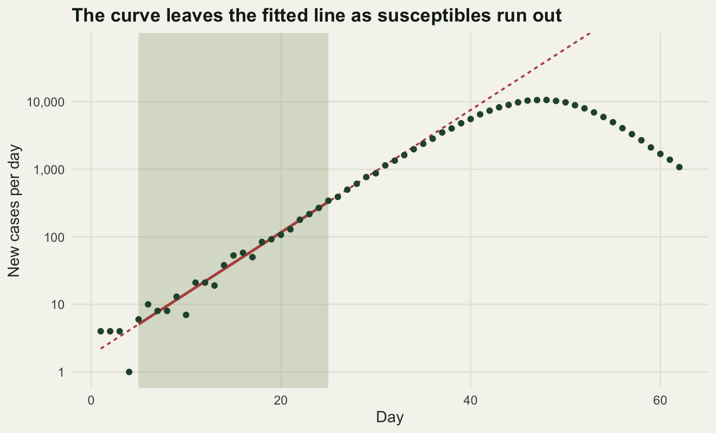
From a growth rate to a reproduction number
The map is one line of mathematics. If incidence grows as \(e^{rt}\) and every case produces \(R_0\) secondary cases spread over the generation interval density \(g\), then consistency requires
\[1 = R_0 \int_0^\infty g(a) e^{-ra} \, da = R_0 \, M(-r),\]
where \(M\) is the moment generating function of the generation interval. So \(R_0 = 1 / M(-r)\). The integral discounts secondary cases by how late they arrive: in a growing epidemic a case produced five days from now is worth less than one produced tomorrow, because by then the whole epidemic has grown. A generation interval that is long, or that has a lot of mass at long delays, therefore demands a larger \(R_0\) to produce the same observed growth.
For a gamma with shape \(k\) and mean \(m\) the integral has a closed form, \(R_0 = (1 + rm/k)^k\). Code the integral numerically anyway and check the two against each other, because the numerical version is the one that will work for an empirical generation interval that has no closed form.
r0_gamma_num <- function(r, shape, gmean) {
  1 / integrate(function(a) exp(-r * a) * dgamma(a, shape = shape, rate = shape / gmean),
                0, Inf, rel.tol = 1e-12)$value
}
r0_gamma_cf <- function(r, shape, gmean) (1 + r * gmean / shape)^shape

r_hat <- fit$coef[2]
round(c(numeric_R0 = r0_gamma_num(r_hat, gi_shape, gi_mean),
        closed_form_R0 = r0_gamma_cf(r_hat, gi_shape, gi_mean)), 6)
numeric_R0 closed_form_R0
2.526446 2.526446 signif(c(numeric_minus_closed_form = abs(r0_gamma_num(r_hat, gi_shape, gi_mean) -
r0_gamma_cf(r_hat, gi_shape, gi_mean))), 3)numeric_minus_closed_form
8.88e-16 round(c(R0_from_true_r_discrete = r0_from_r(r_true, w_true),
R0_from_true_r_continuous = r0_gamma_cf(r_true, gi_shape, gi_mean),
R0_from_fitted_r = r0_from_r(r_hat, w_true)), 5) R0_from_true_r_discrete R0_from_true_r_continuous R0_from_fitted_r
2.50000 2.50161 2.52476 The two agree to 8.88e-16, which is machine noise, and the map is exact where it should be: feeding the true growth rate through the true discretised generation interval returns 2.5 to five decimal places, and through the continuous gamma returns 2.50161. The fitted growth rate returns 2.52476, so the estimation error in \(r\) costs about one per cent in \(R_0\).
That is the easy part. Now the part that is not measured in most wildlife outbreaks. Hold the growth rate fixed at the value just estimated, hold the mean generation interval fixed at 5 days, and change only the shape of the distribution: exponential, gamma with shape 4, and a fixed delay with no variation at all.
r0_fixed_delay <- function(r, gmean) exp(r * gmean)

three_shapes <- c(exponential = r0_gamma_cf(r_hat, 1, gi_mean),
                  gamma_shape_4 = r0_gamma_cf(r_hat, gi_shape, gi_mean),
                  fixed_delay = r0_fixed_delay(r_hat, gi_mean))
mean_sweep <- c(mean_minus_20pc = r0_gamma_cf(r_hat, gi_shape, 0.8 * gi_mean),
                mean_as_assumed = r0_gamma_cf(r_hat, gi_shape, gi_mean),
                mean_plus_20pc = r0_gamma_cf(r_hat, gi_shape, 1.2 * gi_mean))

round(three_shapes, 4)
exponential gamma_shape_4 fixed_delay
2.0430 2.5264 2.8377 round(mean_sweep, 4)mean_minus_20pc mean_as_assumed mean_plus_20pc
2.1337 2.5264 2.9711 round(c(shape_spread_ratio = max(three_shapes) / min(three_shapes),
mean_spread_ratio = as.numeric(mean_sweep[3] / mean_sweep[1]),
mean_swept_by_pc = 20), 4)shape_spread_ratio mean_spread_ratio mean_swept_by_pc
1.3890 1.3925 20.0000 r_fast <- 2 * r_hat
fast_shapes <- c(r0_gamma_cf(r_fast, 1, gi_mean), r0_gamma_cf(r_fast, gi_shape, gi_mean),
r0_fixed_delay(r_fast, gi_mean))
fast_means <- c(r0_gamma_cf(r_fast, gi_shape, 0.8 * gi_mean),
r0_gamma_cf(r_fast, gi_shape, 1.2 * gi_mean))
thresholds <- 1 - 1 / three_shapes
round(thresholds, 4) exponential gamma_shape_4 fixed_delay
0.5105 0.6042 0.6476 round(c(threshold_gap_percentage_points = 100 * (max(thresholds) - min(thresholds))), 4)threshold_gap_percentage_points
13.7078 round(c(faster_r = r_fast,
fast_shape_spread = max(fast_shapes) / min(fast_shapes),
fast_mean_spread = fast_means[2] / fast_means[1]), 4) faster_r fast_shape_spread fast_mean_spread
0.4172 2.6093 1.7320 One growth rate, three answers. An exponential generation interval gives 2.043, a gamma with shape 4 gives 2.5264, and a fixed delay gives 2.8377, a spread of a factor of 1.389 across assumptions that all agree on the mean. The ordering is not arbitrary. A fixed delay puts every secondary case at exactly 5 days, the most heavily discounted position available; the exponential puts a lot of mass at short delays, where cases are cheap, so it needs the smallest \(R_0\) to explain the same growth. Variability in the generation interval pulls \(R_0\) towards one.
Now the other assumption. Keep the shape at 4 and move the mean by plus and minus 20 per cent, a modest amount of ignorance about a quantity nobody measured. \(R_0\) runs from 2.1337 to 2.9711, a factor of 1.3925.
The two are nearly equal, which is not what I expected. The received advice is that the shape of the generation interval is a detail and its mean is what matters, and at this growth rate the two sources of error are within half a per cent of each other in their effect. The tie is a property of this growth rate, though, not a general result. Double the growth rate to 0.4172 per day and the shape spread widens to 2.6093 while the mean spread only reaches 1.732. The reason is in the formulas: the fixed delay answer grows exponentially in \(rm\), the exponential answer only linearly, so the gap between them opens as the epidemic gets faster. For a slow wildlife epidemic the mean is the thing to argue about. For a fast one the shape is.
None of this stays inside the model. The fraction of the host population that has to be immune to hold transmission below threshold is \(1 - 1/R_0\), so the same three assumptions give 0.5105, 0.6042 and 0.6476: a gap of 13.7078 percentage points of vaccination or cull coverage, decided by the shape of a distribution that was not measured. R0 and herd immunity works through what that threshold does and does not promise.
mgrid <- seq(3, 7, length.out = 120)
gi_curves <- rbind(
  data.frame(gmean = mgrid, R0 = r0_gamma_cf(r_hat, 1, mgrid),
             assumption = "Exponential"),
  data.frame(gmean = mgrid, R0 = r0_gamma_cf(r_hat, gi_shape, mgrid),
             assumption = "Gamma, shape 4"),
  data.frame(gmean = mgrid, R0 = r0_fixed_delay(r_hat, mgrid),
             assumption = "Fixed delay"))
gi_curves$assumption <- factor(gi_curves$assumption,
                               levels = c("Exponential", "Gamma, shape 4", "Fixed delay"))
marks <- data.frame(gmean = gi_mean, R0 = as.numeric(three_shapes),
                    assumption = factor(levels(gi_curves$assumption),
                                        levels = levels(gi_curves$assumption)))

ggplot(gi_curves, aes(gmean, R0, colour = assumption)) +
  annotate("rect", xmin = 0.8 * gi_mean, xmax = 1.2 * gi_mean,
           ymin = -Inf, ymax = Inf, fill = te_pal$sage, alpha = 0.25) +
  geom_hline(yintercept = r0_true, colour = te_pal$ink,
             linetype = "22", linewidth = 0.6) +
  geom_line(linewidth = 0.9) +
  geom_point(data = marks, size = 2.6) +
  scale_colour_manual(values = c(te_pal$green, te_pal$forest, te_pal$clay), name = NULL) +
  labs(x = "Assumed generation interval mean, days", y = "Implied R0",
       title = "One growth rate, three generation intervals") +
  theme_te() +
  theme(legend.position = "top")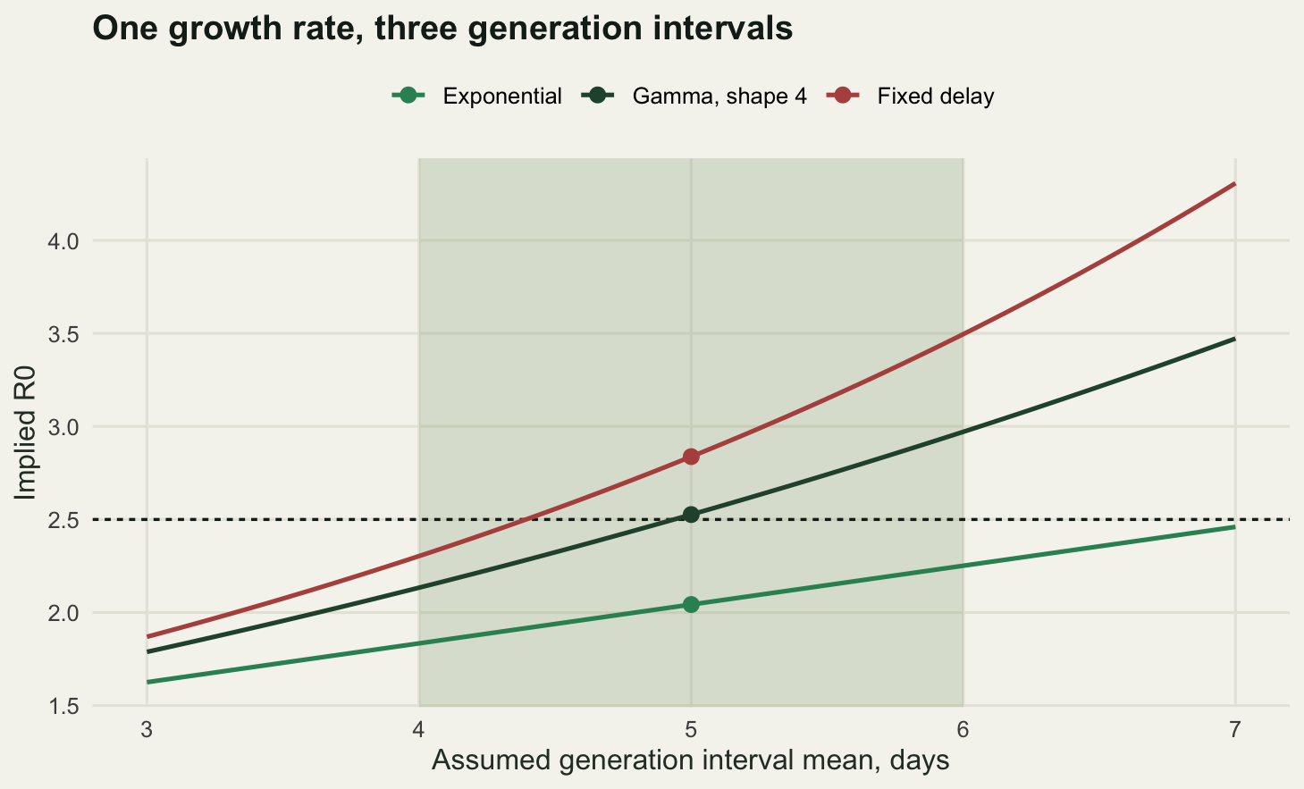
How long a window can you fit?
The exponential phase is a phase, not a property of the epidemic. As susceptibles are used up the per case reproduction number falls to \(R_0 S_t / N\), the curve bends down, and a straight line fitted through the bend has a slope that is too shallow. The estimate of \(R_0\) inherits the bias. Fitting a longer window buys precision and pays in accuracy, so the sweep below fits every window that starts on day 5 and ends anywhere from day 16 to day 55.
ends <- 16:55
sweep <- do.call(rbind, lapply(ends, function(te) {
  sub <- epi[epi$day >= d0 & epi$day <= te, ]
  ff <- irls_pois(sub$inc, sub$day)
  data.frame(end_day = te, window_days = te - d0 + 1, r = ff$coef[2], se = ff$se[2],
             R0 = r0_from_r(ff$coef[2], w_true), sfrac = epi$sfrac[te])
}))
sweep$bias_pc <- 100 * (sweep$R0 / r0_true - 1)

print(round(sweep[sweep$end_day %in% c(16, 20, 25, 30, 35, 40, 44, 50, 55),
                  c("end_day", "window_days", "r", "se", "R0", "sfrac", "bias_pc")], 4))
end_day window_days r se R0 sfrac bias_pc
x 16 12 0.2258 0.0212 2.7012 0.9989 8.0490
x4 20 16 0.2018 0.0112 2.4580 0.9975 -1.6800
x9 25 21 0.2086 0.0058 2.5248 0.9930 0.9903
x14 30 26 0.2058 0.0032 2.4973 0.9800 -0.1071
x19 35 31 0.2018 0.0018 2.4575 0.9452 -1.7003
x24 40 36 0.1912 0.0011 2.3556 0.8575 -5.7756
x28 44 40 0.1746 0.0007 2.2016 0.7194 -11.9378
x34 50 46 0.1320 0.0004 1.8419 0.4166 -26.3251
x39 55 51 0.0921 0.0003 1.5465 0.2191 -38.1383first_bad <- which(sweep$bias_pc < -10)[1]
round(c(shortest_window = min(sweep$window_days),
bias_at_shortest = sweep$bias_pc[1],
se_at_shortest = sweep$se[1],
se_at_longest = sweep$se[nrow(sweep)]), 4) shortest_window bias_at_shortest se_at_shortest se_at_longest
12.0000 8.0490 0.0212 0.0003 round(c(first_window_past_10pc = sweep$window_days[first_bad],
its_end_day = sweep$end_day[first_bad],
pc_below_truth_there = -sweep$bias_pc[first_bad],
susceptibles_left = sweep$sfrac[first_bad],
already_infected_pc = 100 * (1 - sweep$sfrac[first_bad]),
pc_below_truth_at_end = -sweep$bias_pc[nrow(sweep)]), 4)first_window_past_10pc its_end_day pc_below_truth_there
40.0000 44.0000 11.9378
susceptibles_left already_infected_pc pc_below_truth_at_end
0.7194 28.0610 38.1383 The shortest window, 12 days, gives a bias of 8.049 per cent with a standard error on the growth rate of 0.0212; that is sampling noise, and the sign flips from realisation to realisation. Between day 20 and day 35 the estimate stays within a few per cent of the truth. After that the bias is one directional and grows: the first window whose estimate falls more than 10 per cent below the truth is 40 days long, ending on day 44, at which point 28.0610 per cent of the population has already been infected and the estimate is 11.9378 per cent below the truth.
The transferable version of that measurement is the susceptible fraction, not the window length, because the window length depends on how fast the epidemic is. Once about a quarter of the host population has been through the infection the exponential growth estimate is out by more than a tenth, and it keeps getting worse while the standard error keeps getting smaller. By day 55 the standard error has fallen to 0.0003 from 0.0212 at the short window, while the point estimate has dropped to 38.1383 per cent below the truth. A tight interval around a badly chosen window is the failure mode to watch for here, because everything in the output looks better as it gets worse.
ggplot(sweep, aes(end_day, R0)) +
  annotate("rect", xmin = -Inf, xmax = Inf, ymin = 0.9 * r0_true, ymax = 1.1 * r0_true,
           fill = te_pal$sage, alpha = 0.25) +
  geom_hline(yintercept = r0_true, colour = te_pal$ink,
             linetype = "22", linewidth = 0.6) +
  geom_line(colour = te_pal$forest, linewidth = 0.8) +
  geom_point(aes(colour = sfrac), size = 2.4) +
  scale_colour_gradient(low = te_pal$gold, high = te_pal$forest,
                        name = "Susceptible fraction") +
  labs(x = "Last day in the fitting window", y = "Estimated R0",
       title = "A longer window returns a smaller reproduction number") +
  theme_te() +
  theme(legend.position = "top")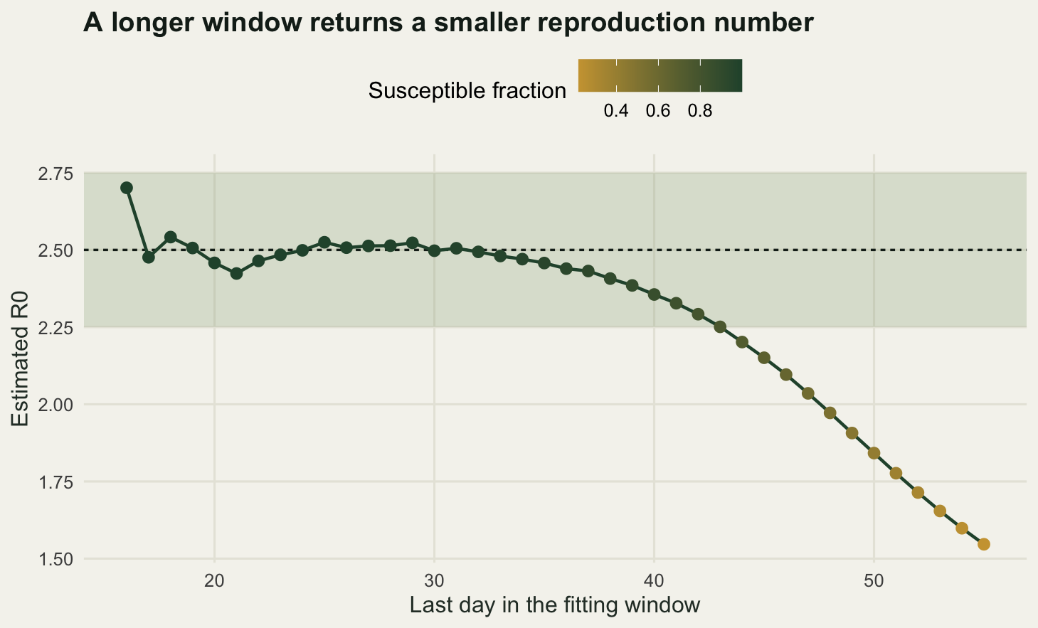
A reproduction number that moves
Once control measures arrive, or once depletion bites, a single number for the whole outbreak is the wrong object. The renewal equation gives a time-varying one directly from its definition: the cases seen on day \(t\) divided by the infectious pressure that produced them,
\[\hat{R}_t = \frac{I_t}{\sum_s w_s I_{t-s}}.\]
Nothing is fitted. The estimate is a ratio, and its noise is the Poisson noise in a single day’s count, which for a small outbreak is a lot of noise. The standard repair is a sliding window: sum the numerator and the denominator over the last \(\tau\) days before dividing. That is the estimator in Cori et al. 2013, written here in its maximum likelihood form: under a flat prior that ratio is the posterior mode, not the posterior mean.
Two properties of that denominator are worth holding on to. It is a sum over past incidence, so the estimate does not exist until enough days have accumulated for the generation interval to have support, and any estimate for the first few days of an outbreak is really a statement about the seeds. It also treats every case in the numerator as having been infected locally. A steady trickle of introductions from outside the population inflates the numerator without contributing to the denominator, so the estimate reads high, and it reads highest when incidence is low and one imported case is a large fraction of a day’s total. That is precisely the situation, the tail end of an outbreak, in which a manager most wants to know whether transmission has stopped.
To measure what the window costs, simulate an outbreak in which the reproduction number steps down on a known day, as it would after a cull, a vaccination campaign or a movement restriction.
lam_of <- function(inc, w) {
  sapply(seq_along(inc), function(t) {
    k <- min(length(w), t - 1)
    if (k < 1) return(NA_real_)
    sum(w[1:k] * inc[t - (1:k)])
  })
}

rt_est <- function(inc, w, tau) {
  lam <- lam_of(inc, w)
  sapply(seq_along(inc), function(t) {
    if (t < tau + 1) return(NA_real_)
    idx <- (t - tau + 1):t
    if (any(is.na(lam[idx])) || sum(lam[idx]) <= 0) return(NA_real_)
    sum(inc[idx]) / sum(lam[idx])
  })
}

step_day <- 24; rt_before <- 2.5; rt_after <- 0.8; tau <- 7; n_days2 <- 60
rt_path <- ifelse(seq_len(n_days2) < step_day, rt_before, rt_after)
set.seed(22)
ep2 <- sim_epi(500000, rep(2, 3), rt_path, w_true, n_days2)
rt7 <- rt_est(ep2$inc, w_true, tau)
rt1 <- rt_est(ep2$inc, w_true, 1)

cross_day <- function(x) {
  ok <- which(!is.na(x) & x < 1 & seq_along(x) > 12)
  if (length(ok) == 0) NA_real_ else ok[1]
}
settle_day <- function(x) {
  ok <- which(!is.na(x) & seq_along(x) >= step_day & abs(x / rt_after - 1) < 0.1)
  if (length(ok) == 0) NA_real_ else ok[1]
}

round(c(true_step_day = step_day, Rt_before = rt_before, Rt_after = rt_after,
        smoothing_window = tau, cases_on_step_day = ep2$inc[step_day],
        peak_cases = max(ep2$inc),
        min_susceptible_fraction = min(ep2$sfrac)), 4)
true_step_day Rt_before Rt_after
24.0000 2.5000 0.8000
smoothing_window cases_on_step_day peak_cases
7.0000 81.0000 210.0000
min_susceptible_fraction
0.9942 round(c(crossing_day_smoothed = cross_day(rt7), crossing_day_unsmoothed = cross_day(rt1),
lag_smoothed = cross_day(rt7) - step_day,
lag_unsmoothed = cross_day(rt1) - step_day,
settles_within_10pc_on_day = settle_day(rt7)), 3) crossing_day_smoothed crossing_day_unsmoothed
30 24
lag_smoothed lag_unsmoothed
6 0
settles_within_10pc_on_day
30 round(c(Rt_on_step_day = rt7[step_day], Rt_one_day_after = rt7[step_day + 1],
Rt_two_days_after = rt7[step_day + 2],
bias_pc_one_day_after = 100 * (rt7[step_day + 1] / rt_after - 1)), 3) Rt_on_step_day Rt_one_day_after Rt_two_days_after
2.282 1.857 1.561
bias_pc_one_day_after
132.086 round(c(sd_unsmoothed_growth_phase = sd(rt1[14:23]),
sd_smoothed_growth_phase = sd(rt7[14:23]),
noise_ratio = sd(rt1[14:23]) / sd(rt7[14:23])), 4)sd_unsmoothed_growth_phase sd_smoothed_growth_phase
0.3074 0.0868
noise_ratio
3.5433 The outbreak carries 81 cases on the day of the step and peaks at 210, small enough that the unsmoothed estimator is visibly noisy: its standard deviation over the growth phase is 0.3074 against a true value of 2.5, while the seven day version scatters by 0.0868, a factor of 3.5433 less. That is the case for smoothing.
The cost is on the other side of the step. The unsmoothed estimator crosses one on day 24, the day the step happened, with no lag at all, because its numerator is the first post-step day of cases and its denominator is the pre-step pressure that generated them. The seven day estimator crosses on day 30, a lag of 6 days. One day after the step it reads 1.857 against a truth of 0.8, which is 132.086 per cent too high, and it does not come within 10 per cent of the new value until day 30. The window has not smoothed the estimate, it has averaged over a period during which the reproduction number took two different values: on the step day itself, six of the seven days in the window are still pre-step, and they drag the average up.
A six day lag is a long time in an outbreak with a doubling time of about three days. If the estimate is being used to decide whether an intervention worked, a seven day window will report failure for most of a week after it succeeded. The window length is a choice between two errors and there is no setting that avoids both; what you can do is report the window alongside the estimate, and never read a turning point off a smoothed series without allowing the lag.
rt_long <- rbind(
  data.frame(day = ep2$day, Rt = rt1, series = "Unsmoothed"),
  data.frame(day = ep2$day, Rt = rt7, series = "Seven day window"))
rt_long <- rt_long[!is.na(rt_long$Rt) & rt_long$day >= 11 & rt_long$day <= 50, ]
rt_long$series <- factor(rt_long$series, levels = c("Unsmoothed", "Seven day window"))
truth_line <- data.frame(day = ep2$day, Rt = rt_path)
truth_line <- truth_line[truth_line$day >= 11 & truth_line$day <= 50, ]

ggplot(rt_long, aes(day, Rt, colour = series, linewidth = series)) +
  geom_hline(yintercept = 1, colour = te_pal$line, linewidth = 0.9) +
  geom_step(data = truth_line, aes(day, Rt), inherit.aes = FALSE,
            colour = te_pal$ink, linetype = "22", linewidth = 0.7) +
  geom_line() +
  scale_colour_manual(values = c(te_pal$green, te_pal$clay), name = NULL) +
  scale_linewidth_manual(values = c(0.8, 1.1), guide = "none") +
  coord_cartesian(ylim = c(0, 4)) +
  labs(x = "Day", y = "Reproduction number",
       title = "The smoothed estimate finds the step late") +
  theme_te() +
  theme(legend.position = "top")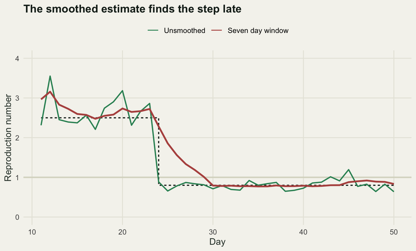
The left hand end of that figure shows the other property of the denominator at work. The earliest estimates sit above the true value, because the seeded cases arrived from outside and have no history behind them to divide by, and the bias fades only once locally generated cases dominate the sum. An outbreak that keeps receiving introductions never leaves that regime.
The honest limit: what cumulative counts do to the interval
Incidence is sometimes hard to get and a cumulative curve is easy, because the total number of cases to date is the number that gets reported. Fitting the same log-linear model to cumulative counts looks harmless. The cumulative total of an exponentially growing series grows at the same rate, so the slope estimates the same quantity, and the counts are larger, so the interval comes back tighter. Both halves of that sentence are true and the conclusion is wrong.
cum_all <- cumsum(epi$inc)
fit_cum <- irls_pois(cum_all[epi$day >= d0 & epi$day <= d1], early$day)

round(c(r_from_incidence = fit$coef[2], se_incidence = as.numeric(fit$se[2]),
        r_from_cumulative = fit_cum$coef[2],
        se_cumulative = as.numeric(fit_cum$se[2]), r_true = r_true), 5)
r_from_incidence se_incidence r_from_cumulative se_cumulative
0.20860 0.00579 0.21328 0.00257
r_true
0.20611 round(c(confidence_level_pc = 95,
ci_width_incidence = as.numeric(2 * 1.96 * fit$se[2]),
ci_width_cumulative = as.numeric(2 * 1.96 * fit_cum$se[2]),
width_ratio = as.numeric(fit_cum$se[2] / fit$se[2])), 4)confidence_level_pc ci_width_incidence ci_width_cumulative width_ratio
95.0000 0.0227 0.0101 0.4443 On this outbreak the cumulative fit returns 0.21328 against the incidence fit’s 0.20860 and a truth of 0.20611. Its 95 per cent interval is 0.0101 wide against 0.0227 for incidence, a ratio of 0.4443. The cumulative interval is less than half the width and it does not contain the truth. One realisation proves nothing, so run the whole thing 400 times.
n_rep <- 400
set.seed(909)
cov_tab <- do.call(rbind, lapply(seq_len(n_rep), function(i) {
  ee <- sim_epi(n_pop, rep(n_seed, 3), rep(r0_true, d1 + 5), w_true, d1 + 5)
  sub <- ee[ee$day >= d0 & ee$day <= d1, ]
  cc <- cumsum(ee$inc)[ee$day >= d0 & ee$day <= d1]
  a <- irls_pois(sub$inc, sub$day)
  b <- irls_pois(cc, sub$day)
  data.frame(ri = a$coef[2], si = a$se[2], rc = b$coef[2], sc = b$se[2])
}))

round(c(replicates = n_rep,
        coverage_incidence = mean(abs(cov_tab$ri - r_true) < 1.96 * cov_tab$si),
        coverage_cumulative = mean(abs(cov_tab$rc - r_true) < 1.96 * cov_tab$sc),
        nominal = 0.95), 4)
replicates coverage_incidence coverage_cumulative nominal
400.00 0.93 0.39 0.95 round(c(median_width_incidence = median(2 * 1.96 * cov_tab$si),
median_width_cumulative = median(2 * 1.96 * cov_tab$sc),
median_width_ratio = median(cov_tab$sc / cov_tab$si)), 4) median_width_incidence median_width_cumulative median_width_ratio
0.0232 0.0103 0.4428 round(c(mean_r_incidence = mean(cov_tab$ri), mean_r_cumulative = mean(cov_tab$rc),
bias_pc_incidence = 100 * (mean(cov_tab$ri) / r_true - 1),
bias_pc_cumulative = 100 * (mean(cov_tab$rc) / r_true - 1)), 4) mean_r_incidence mean_r_cumulative bias_pc_incidence bias_pc_cumulative
0.2049 0.2107 -0.5873 2.2060 round(c(actual_sd_incidence = sd(cov_tab$ri), reported_se_incidence = mean(cov_tab$si),
actual_sd_cumulative = sd(cov_tab$rc), reported_se_cumulative = mean(cov_tab$sc),
sd_over_se_incidence = sd(cov_tab$ri) / mean(cov_tab$si),
sd_over_se_cumulative = sd(cov_tab$rc) / mean(cov_tab$sc)), 4) actual_sd_incidence reported_se_incidence actual_sd_cumulative
0.0065 0.0060 0.0081
reported_se_cumulative sd_over_se_incidence sd_over_se_cumulative
0.0027 1.0810 3.0506 Across 400 replicate outbreaks the incidence interval covers the truth 0.93 of the time against a nominal 0.95, which is the small overdispersion you would expect from a renewal process fitted as if the counts were independent Poisson draws. The cumulative interval covers 0.39 of the time. Its median width is 0.4428 of the incidence interval, so it is not merely wrong, it is confidently wrong.
The three ingredients are separable. The cumulative estimator is biased: it averages 0.2107 against a truth of 0.20611, 2.2060 per cent high, because the seeded cases sit in the cumulative total from day one and flatten its early slope, which the fit compensates for with a steeper one later. It is also less precise than it looks: the actual spread of its estimates across replicates is 0.0081, while the standard error it reports averages 0.0027, so the reported interval is 3.0506 times too narrow. The incidence version has the same ratio at 1.0810, and its point estimates average 0.2049 against the same truth. The reason for both is that successive cumulative counts are almost the same number, since \(C_t = C_{t-1} + I_t\) and \(I_t\) is a small fraction of \(C_{t-1}\), so the 21 data points carry nothing like 21 independent pieces of information, while the Poisson likelihood counts them as if they did.
The rule that comes out of this is short. Fit incidence. If only a cumulative series exists, difference it first and accept the noise, because the noise is real and the smoothness is an artefact.
There is a limit around all of this that no amount of care with the estimator removes. Every number above was computed on a simulation in which cases are observed the day they are infected, with no reporting delay, no under-detection that varies through the outbreak, and no imported cases after day three. In a real wildlife system, cases are found when someone goes looking, detection effort rises once an outbreak is recognised, and rising effort mimics rising transmission exactly. The generation interval used in the map was the one that generated the data. If it were estimated from contact tracing during the growth phase it would be biased short, which by the generation interval sweep would push \(R_0\) towards one. What the method delivers is a reproduction number conditional on an observation process and a generation interval, and both belong in the sentence that reports it.
Where to go next
The reproduction number estimated here is a summary of transmission at one moment in one population. What it implies over years depends on how susceptibles are replenished, and a number above one does not by itself predict a recurrent epidemic: seasonality and recurrent epidemics takes the same machinery into repeated outbreaks and asks when transmission has to be forced to keep them going. The estimates in this post came out close to the truth because the truth was available to check them against, which is the one thing a real outbreak never supplies; checking an epidemic estimate is the set of diagnostics that stands in for it.
References
Wallinga J, Lipsitch M 2007 Proceedings of the Royal Society B 274(1609):599-604 (10.1098/rspb.2006.3754)
Cori A, Ferguson NM, Fraser C, Cauchemez S 2013 American Journal of Epidemiology 178(9):1505-1512 (10.1093/aje/kwt133)
Wallinga J, Teunis P 2004 American Journal of Epidemiology 160(6):509-516 (10.1093/aje/kwh255)
Ma J, Dushoff J, Bolker BM, Earn DJD 2014 Bulletin of Mathematical Biology 76(1):245-260 (10.1007/s11538-013-9918-2)