library(ggplot2)
library(patchwork)
library(splines)

te_paper  <- "#f5f4ee"
te_ink    <- "#16241d"
te_body   <- "#2c3a31"
te_forest <- "#275139"
te_rust   <- "#b5534e"
te_gold   <- "#c9b458"
te_line   <- "#dad9ca"

theme_datasheet <- function() {
  theme_minimal(base_size = 12) +
    theme(plot.background  = element_rect(fill = te_paper, colour = NA),
          panel.background = element_rect(fill = te_paper, colour = NA),
          panel.grid.major = element_line(colour = te_line, linewidth = 0.3),
          panel.grid.minor = element_blank(),
          text             = element_text(colour = te_body),
          plot.title       = element_text(colour = te_ink, face = "bold"),
          plot.subtitle    = element_text(colour = te_body),
          axis.text        = element_text(colour = te_body),
          strip.text       = element_text(colour = te_ink, face = "bold"))
}Self-exciting events and the Hawkes process
R
point processes
time series
acoustic monitoring
statistics
ecology tutorial
A clustered event series fits a Hawkes process and a changing background rate alike. Simulating, fitting and checking both in R shows when time separates them.
An autonomous recorder sits at the edge of a reed bed for forty days and logs every detection of one species’ territorial call. Plotted along a time axis, the detections are not spread evenly. They come in bursts: several calls within a quarter of an hour, then long quiet stretches. Two stories fit that picture. In the first, one bird calling provokes a neighbour to answer, so each call raises the chance of another call for a short while; the process excites itself. In the second, the birds call independently of one another, but the calling rate rises and falls with the weather, so there are good hours and bad hours and the detections pile up in the good ones. Carcass finds in a disease survey, landslides after rain and strandings along a coast raise exactly the same question.
The spatial version of this question has already appeared on this site. Modelling inhomogeneous point patterns in R simulates a pattern whose density follows a gradient and shows that a homogeneous Ripley’s K calls it clustered. Its closing warning reads: “There is a genuine identifiability tension between a smoothly varying intensity and short-range clustering, because both put extra points close together, and no amount of arithmetic fully resolves it from a single pattern.” In space the only lever is a difference in scale between the trend and the clustering. Time keeps that lever, since the excitation decays over minutes while the weather changes over days, and adds a second one: if a call provokes calls, the extra events follow earlier events and never precede them. This post measures how far the scale lever goes in time; it does not isolate what the direction adds.
The tool is the Hawkes process, in which the conditional intensity at time t is a background rate plus a sum of decaying kicks, one for every earlier event. It is a close relative of the renewal equation in estimating R0 from incidence data: the branching ratio of a Hawkes process is the expected number of direct offspring per event, the same quantity a reproduction number measures, and a ratio below one keeps the process from exploding. It is a different model from the shared frailty in frailty and recurrent event models, where events cluster because some individuals have a higher fixed rate; nothing there makes one event cause the next.
The post writes the simulator (Ogata’s thinning) and the likelihood (Ozaki’s recursion for an exponential kernel) in base R and checks both against brute force. It then crosses the two stories with the two models: a background that swings slowly fitted with a Hawkes model that has a constant background, and a genuinely self-exciting series fitted with a smooth background and no excitation. It measures how far a Hawkes model with a flexible background separates them, and where that separation breaks. Finally it checks the fits with residuals from time rescaling, and finds that the usual gap-based checks see one of the two mistakes and are blind to the other, while a count of rescaled events in blocks of a suitable length sees the second one some of the time.
Simulating by thinning, fitting by recursion
The model has a background rate mu(t) and an exponential kernel. After an event at time s the intensity is raised by alpha exp(-beta (t - s)), so each event adds alpha / beta expected direct offspring over an unbounded horizon. That ratio is the branching ratio, written n below, and the post fits the model in terms of n and beta rather than alpha and beta for a reason that the validation shows. The design constants are fixed here before anything is run: a window of 960 hours, a background of 0.4 detections per hour, a branching ratio of 0.4 and a decay rate of 2 per hour, so a provoked call follows its parent after half an hour on average.
Simulation uses Ogata’s thinning. Between events the excitation only decays, so the intensity just after the current time bounds the intensity until the next accepted event. A candidate waiting time is drawn from that bound, the excitation is decayed over the wait, and the candidate is kept with probability equal to the true intensity over the bound. A rejected candidate still moves the clock forward, which is what makes the method exact. For a background that varies, the bound uses the maximum of the background.
T_end     <- 960   # hours of recording
mu0       <- 0.4   # background detections per hour
br_true   <- 0.4   # branching ratio n = alpha / beta
beta_true <- 2     # kernel decay per hour
amp       <- 1     # log amplitude of the slow background wave
P0        <- 240   # period of the slow background wave, hours
k_flex    <- 16    # spline basis size for the flexible background

sim_hawkes <- function(mu_fun, mu_max, br, beta, t_max = T_end) {
  alpha <- br * beta
  ev <- numeric(0); s_now <- 0; exc <- 0
  repeat {
    lam_bar <- mu_max + exc
    wait <- rexp(1, lam_bar)
    if (s_now + wait > t_max) break
    exc <- exc * exp(-beta * wait)
    s_now <- s_now + wait
    if (runif(1) * lam_bar <= mu_fun(s_now) + exc) {
      ev <- c(ev, s_now)
      exc <- exc + alpha
    }
  }
  ev
}
bg_flat <- function(level) function(s) rep(level, length(s))
bg_wave <- function(P) function(s) mu0 * exp(amp * sin(2 * pi * s / P))

# Ozaki recursion: A_i = sum_{j<i} exp(-beta (t_i - t_j)); B_i = dA_i / dbeta
rec_AB <- function(tt, beta) {
  n_ev <- length(tt); A <- numeric(n_ev); B <- numeric(n_ev)
  if (n_ev > 1) for (i in 2:n_ev) {
    gap <- tt[i] - tt[i - 1]; e_gap <- exp(-beta * gap)
    B[i] <- e_gap * (B[i - 1] - gap * (1 + A[i - 1]))
    A[i] <- e_gap * (1 + A[i - 1])
  }
  list(A = A, B = B)
}

n_grid <- 960
make_basis <- function(tt, k) {
  mid <- (seq_len(n_grid) - 0.5) * T_end / n_grid
  if (k == 1) return(list(Xg = matrix(1, n_grid, 1), Xe = matrix(1, length(tt), 1),
                          dt = T_end / n_grid, k = 1))
  bb <- bs(mid, df = k, intercept = TRUE, Boundary.knots = c(0, T_end))
  list(Xg = unclass(bb)[, 1:k], Xe = unclass(predict(bb, tt))[, 1:k, drop = FALSE],
       dt = T_end / n_grid, k = k)
}

# negative log likelihood and gradient; par = (spline coefs, n, log beta)
nll_grad <- function(par, tt, bas, hawkes = TRUE) {
  k <- bas$k; th <- par[1:k]
  mu_e <- exp(drop(bas$Xe %*% th)); mu_g <- exp(drop(bas$Xg %*% th))
  bg_int <- sum(mu_g) * bas$dt
  if (!hawkes) return(list(val = -(sum(log(mu_e)) - bg_int),
    grad = -(colSums(bas$Xe) - colSums(bas$Xg * mu_g) * bas$dt)))
  nb <- par[k + 1]; beta <- exp(par[k + 2])
  ab <- rec_AB(tt, beta)
  lam <- mu_e + nb * beta * ab$A
  rem <- T_end - tt; e_rem <- exp(-beta * rem)
  ll <- sum(log(lam)) - bg_int - nb * sum(1 - e_rem)      # compensator included
  g_th <- colSums(bas$Xe * (mu_e / lam)) - colSums(bas$Xg * mu_g) * bas$dt
  g_n  <- sum(beta * ab$A / lam) - sum(1 - e_rem)
  g_lb <- sum(nb * beta * (ab$A + beta * ab$B) / lam) - nb * sum(rem * beta * e_rem)
  list(val = -ll, grad = -c(g_th, g_n, g_lb))
}

fit_pp <- function(tt, k, hawkes = TRUE) {
  bas <- make_basis(tt, k); lvl <- log(length(tt) / T_end)
  if (!hawkes) {
    o <- optim(rep(lvl, k), function(p) nll_grad(p, tt, bas, FALSE)$val,
               function(p) nll_grad(p, tt, bas, FALSE)$grad,
               method = "BFGS", control = list(maxit = 1000))
  } else {
    o <- NULL
    for (b_start in c(1, 0.05)) {           # two starts: fast and slow kernel
      o_try <- optim(c(rep(lvl + log(0.7), k), 0.3, log(b_start)),
                     function(p) nll_grad(p, tt, bas)$val,
                     function(p) nll_grad(p, tt, bas)$grad, method = "L-BFGS-B",
                     lower = c(rep(-20, k), 0, log(0.01)),
                     upper = c(rep(10, k), 0.98, log(200)),
                     control = list(maxit = 1000))
      if (is.null(o) || o_try$value < o$value) o <- o_try
    }
  }
  o$bas <- bas; o$k <- k; o$hawkes <- hawkes; o$tt <- tt
  o$n_hat <- if (hawkes) o$par[k + 1] else 0
  o$beta_hat <- if (hawkes) exp(o$par[k + 2]) else NA
  o
}

# compensator Lambda(t_i): background integral plus n ((i - 1) - A_i)
compensator <- function(f) {
  tt <- f$tt; mu_g <- exp(drop(f$bas$Xg %*% f$par[1:f$k]))
  cum <- c(0, cumsum(mu_g) * f$bas$dt)
  edges <- seq(0, T_end, length.out = n_grid + 1)
  cell <- pmin(findInterval(tt, edges), n_grid)
  base <- cum[cell] + mu_g[cell] * (tt - edges[cell])
  if (!f$hawkes) return(base)
  base + f$n_hat * ((seq_along(tt) - 1) - rec_AB(tt, f$beta_hat)$A)
}
The recursion is what makes the likelihood cheap. The log likelihood of a point process on a window is the sum of the log intensity at the events minus the compensator, the integral of the intensity over the window. With an exponential kernel the sum of kicks felt by event i is exp(-beta gap) times one plus the sum felt by event i - 1, so the whole sum takes one pass through the events instead of a double loop, and the kernel part of the compensator is n times the sum of 1 - exp(-beta (T - t_i)). The background is a B-spline on the log scale; its integral is taken on a grid of 960 one hour cells, and a basis of size one is a constant background. Both the recursion and the compensator are claims until they are checked.
set.seed(2408)
tt_chk <- sim_hawkes(bg_flat(mu0), mu0, br_true, beta_true)
bas_chk <- make_basis(tt_chk, 1)
par_chk <- c(log(mu0), br_true, log(beta_true))
ll_rec <- -nll_grad(par_chk, tt_chk, bas_chk)$val
alpha_true <- br_true * beta_true
lam_brute <- vapply(seq_along(tt_chk), function(i)
  mu0 + sum(alpha_true * exp(-beta_true * (tt_chk[i] - tt_chk[seq_len(i - 1)]))), 0)
ll_brute <- sum(log(lam_brute)) - mu0 * T_end -
  sum(br_true * (1 - exp(-beta_true * (T_end - tt_chk))))
ll_gap <- abs(ll_rec - ll_brute)
g_an <- nll_grad(par_chk, tt_chk, bas_chk)$grad
g_num <- vapply(1:3, function(j) {
  h <- 1e-5; pp <- par_chk; pm <- par_chk; pp[j] <- pp[j] + h; pm[j] <- pm[j] - h
  (nll_grad(pp, tt_chk, bas_chk)$val - nll_grad(pm, tt_chk, bas_chk)$val) / (2 * h) }, 0)
grad_gap <- max(abs(g_an - g_num))
# compensator at the 200th event against numerical integration of the path
f_chk <- list(tt = tt_chk, bas = bas_chk, k = 1, hawkes = TRUE,
              par = par_chk, n_hat = br_true, beta_hat = beta_true)
i_chk <- 200
fine <- seq(0, tt_chk[i_chk], length.out = 400001)
mid_f <- (fine[-1] + fine[-length(fine)]) / 2
past <- tt_chk[seq_len(i_chk - 1)]
kick <- vapply(past, function(s) sum(exp(-beta_true * (mid_f[mid_f > s] - s))), 0)
comp_num <- mu0 * tt_chk[i_chk] + alpha_true * sum(kick) * diff(fine[1:2])
comp_rec <- compensator(f_chk)[i_chk]
n_chk_ev <- length(tt_chk)
On one simulated series of 687 detections, the recursive log likelihood is -781.5994 and the double loop gives -781.5994, an absolute difference of 6.6e-12. The analytic gradient agrees with central differences to 1.5e-07, and the recursive compensator at the 200th event, 174.3861, matches a numerical integral of the intensity path, 174.3823.
n_val <- 200     # fixed before any estimate was inspected
set.seed(2409)
val <- t(replicate(n_val, {
  tt <- sim_hawkes(bg_flat(mu0), mu0, br_true, beta_true)
  f <- fit_pp(tt, 1)
  c(n_ev = length(tt), mu = exp(f$par[1]), n = f$n_hat, beta = f$beta_hat)
}))
count_theory <- mu0 * T_end / (1 - br_true) - mu0 * br_true / (beta_true * (1 - br_true)^2) *
  (1 - exp(-beta_true * (1 - br_true) * T_end))
count_mean <- mean(val[, "n_ev"]); count_se <- sd(val[, "n_ev"]) / sqrt(n_val)
count_z <- (count_mean - count_theory) / count_se
val_mean <- colMeans(val); val_se <- apply(val, 2, sd) / sqrt(n_val)
alpha_hat <- val[, "n"] * val[, "beta"]
cv_alpha <- sd(alpha_hat) / mean(alpha_hat); cv_n <- sd(val[, "n"]) / mean(val[, "n"])
cor_ab <- cor(alpha_hat, val[, "beta"]); cor_nb <- cor(val[, "n"], val[, "beta"])
The simulator has its own check. A Hawkes process started empty has expected count mu T / (1 - n) minus a start-up correction that decays at rate beta (1 - n), which here is 639.8 detections. Over 200 simulated series the mean count is 635.0 with a Monte Carlo standard error of 2.8, -1.67 standard errors from the expectation. Fitting the correct model with a constant background returns a mean background of 0.396 against 0.4, a mean branching ratio of 0.400 (standard error 0.003) against 0.4, and a mean decay rate of 2.00 against 2.
Those fits also show why the branching ratio is the parameter to report. The kick size alpha and the decay rate beta are estimated together: their estimates correlate at 0.79 across replicates, because a larger kick that fades faster produces a similar number of offspring. Their ratio is better determined. The coefficient of variation of alpha is 0.148 and that of n is 0.098, 1.5 times smaller, and the correlation between n and beta is -0.41. The ratio n = alpha / beta is the number of offspring over an unbounded horizon; near the end of the window part of that offspring has not yet happened, which the compensator term handles, but a series only a few kernel lengths long cannot pin it down.
set.seed(2410)
tt_hwk_ex <- sim_hawkes(bg_flat(mu0), mu0, br_true, beta_true)
tt_wav_ex <- sim_hawkes(bg_wave(P0), mu0 * exp(amp), 0, beta_true)
t_show <- 240
path_t <- seq(0, t_show, by = 0.05)
lam_path <- mu0 + vapply(path_t, function(s) {
  past_ev <- tt_hwk_ex[tt_hwk_ex < s]
  sum(alpha_true * exp(-beta_true * (s - past_ev))) }, 0)
lev <- c("self-exciting, constant background", "independent, slow background wave")
path_df <- rbind(data.frame(time = path_t, lam = lam_path, which = lev[1]),
                 data.frame(time = path_t, lam = bg_wave(P0)(path_t), which = lev[2]))
rug_df <- rbind(data.frame(time = tt_hwk_ex[tt_hwk_ex < t_show], which = lev[1]),
                data.frame(time = tt_wav_ex[tt_wav_ex < t_show], which = lev[2]))
path_df$which <- factor(path_df$which, lev); rug_df$which <- factor(rug_df$which, lev)
n_show <- table(rug_df$which)
ggplot(path_df, aes(time, lam)) +
  geom_line(colour = te_forest, linewidth = 0.45) +
  geom_rug(data = rug_df, aes(x = time), inherit.aes = FALSE,
           colour = te_rust, alpha = 0.7, length = unit(0.06, "npc")) +
  facet_wrap(~ which, ncol = 1, scales = "free_y") +
  labs(x = "hours since the recorder was deployed", y = "intensity, detections per hour",
       title = "Two ways to make bursts",
       subtitle = "green: conditional intensity; red ticks: detections") +
  theme_datasheet()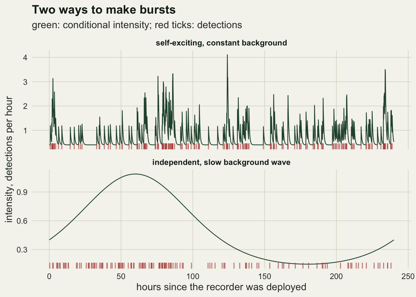
In the first ten days the self-exciting series has 198 detections and the wave series 138. Both look bursty on the rug. The difference is in the green line: in the top panel the intensity jumps at every detection and relaxes within an hour or two, while in the bottom panel it ignores the detections altogether.
A slow background reads as excitation
The first cross fit takes series with no excitation at all, a background that swings between 0.15 and 1.09 detections per hour with a period of 240 hours, and fits a Hawkes model with a constant background. The same simulation loop also generates self-exciting series with a constant background and Poisson series with a constant rate equal to the self-exciting mean, and fits every candidate model to each, so that the later sections reuse one set of replicates.
n_rep <- 100     # fixed before any estimate was inspected
lr_crit <- qchisq(0.95, k_flex - 1)
set.seed(2411)
cross <- t(replicate(n_rep, {
  t_wav <- sim_hawkes(bg_wave(P0), mu0 * exp(amp), 0, beta_true)
  t_hwk <- sim_hawkes(bg_flat(mu0), mu0, br_true, beta_true)
  mu_pois <- mu0 / (1 - br_true)
  t_poi <- sim_hawkes(bg_flat(mu_pois), mu_pois, 0, beta_true)
  wav_h1 <- fit_pp(t_wav, 1); wav_hk <- fit_pp(t_wav, k_flex)
  hwk_p1 <- fit_pp(t_hwk, 1, FALSE); hwk_pk <- fit_pp(t_hwk, k_flex, FALSE)
  hwk_h1 <- fit_pp(t_hwk, 1); hwk_hk <- fit_pp(t_hwk, k_flex)
  poi_p1 <- fit_pp(t_poi, 1, FALSE); poi_pk <- fit_pp(t_poi, k_flex, FALSE)
  swing <- function(f) { m <- exp(drop(f$bas$Xg %*% f$par[1:f$k])); max(m) / min(m) }
  resid <- function(f) {
    lam_c <- compensator(f); gaps <- diff(c(0, lam_c))
    disp_p <- function(blk) {   # dispersion of counts in blocks of blk rescaled units
      cnts <- tabulate(findInterval(lam_c, seq(0, max(lam_c), by = blk)),
                       nbins = floor(max(lam_c) / blk))
      pchisq(sum((cnts - mean(cnts))^2) / mean(cnts), length(cnts) - 1, lower.tail = FALSE)
    }
    c(ks = ks.test(gaps, "pexp")$p.value,
      ac = cor(gaps[-1], gaps[-length(gaps)], method = "spearman"),
      d20 = disp_p(20), d40 = disp_p(40), d80 = disp_p(80))
  }
  c(n_wav_h1 = wav_h1$n_hat, d_wav_h1 = 1 / wav_h1$beta_hat,
    n_wav_hk = wav_hk$n_hat, b_wav_hk = wav_hk$beta_hat,
    n_hwk_h1 = hwk_h1$n_hat, n_hwk_hk = hwk_hk$n_hat,
    swing_hwk = swing(hwk_pk), swing_poi = swing(poi_pk), swing_hwk_hk = swing(hwk_hk),
    lr_bg_hwk = 2 * (hwk_p1$value - hwk_pk$value),
    lr_bg_poi = 2 * (poi_p1$value - poi_pk$value),
    lr_hk_wav = 2 * (wav_h1$value - wav_hk$value),
    lr_hk_hwk = 2 * (hwk_h1$value - hwk_hk$value),
    r_wav_h1 = resid(wav_h1), r_wav_hk = resid(wav_hk),
    r_hwk_pk = resid(hwk_pk), r_hwk_hk = resid(hwk_hk), r_hwk_h1 = resid(hwk_h1))
}))
cm <- colMeans(cross); cse <- apply(cross, 2, sd) / sqrt(n_rep)
q_wav_h1 <- quantile(cross[, "n_wav_h1"], c(0.05, 0.95))
share_zero <- mean(cross[, "n_wav_hk"] < 0.01)
q_d_wav_h1 <- quantile(cross[, "d_wav_h1"], c(0.05, 0.95))
b_zero <- range(cross[cross[, "n_wav_hk"] < 0.01, "b_wav_hk"])
The constant background Hawkes model puts the branching ratio of the wave series at 0.796 on average (Monte Carlo standard error 0.002), with 90 per cent of replicates between 0.760 and 0.834. The true value is zero. The model has no other way to put more detections into a good day than to let each detection call up the next, and so it reports that four in five detections were provoked by an earlier one. The kernel it fits for them is slow: the mean delay 1 / beta is 9.8 hours on average (90 per cent of replicates between 8.5 and 10.9), against half an hour for the true kernel of the self-exciting series.
Giving the same model a flexible background of 16 spline terms removes the artefact: the mean branching ratio falls to 0.005, and 88 per cent of the fits put it below one hundredth. On those fits the decay rate is not estimated at all. Its estimates range from 0.03 to 0.44 per hour, because with no offspring there is no delay to measure, and a decay rate printed next to a branching ratio of zero should be read as an absence rather than a value.
On the self-exciting series, the flexible background costs something in the other direction. With a constant background the mean branching ratio is 0.399; with 16 spline terms it is 0.372 (standard error 0.005). Part of the excitation has moved into the background.
nh_lev <- c("wave truth, constant background", "wave truth, flexible background",
            "exciting truth, constant background", "exciting truth, flexible background")
nh_df <- data.frame(model = factor(rep(nh_lev, each = n_rep), rev(nh_lev)),
                    n_hat = c(cross[, "n_wav_h1"], cross[, "n_wav_hk"],
                              cross[, "n_hwk_h1"], cross[, "n_hwk_hk"]))
truth_df <- data.frame(model = factor(nh_lev, rev(nh_lev)), truth = c(0, 0, br_true, br_true))
med_df <- aggregate(n_hat ~ model, data = nh_df, FUN = median)
set.seed(2412)
ggplot(nh_df, aes(n_hat, model)) +
  geom_point(position = position_jitter(height = 0.18, width = 0),
             colour = te_forest, alpha = 0.45, size = 1.6) +
  geom_point(data = med_df, shape = 124, size = 9, colour = te_ink) +
  geom_point(data = truth_df, aes(truth, model), shape = 23, size = 3.4,
             fill = te_gold, colour = te_ink) +
  scale_x_continuous(limits = c(0, 1)) +
  labs(x = "estimated branching ratio", y = NULL,
       title = "A slow wave looks like excitation",
       subtitle = "gold diamond: true value; black bar: median") +
  theme_datasheet()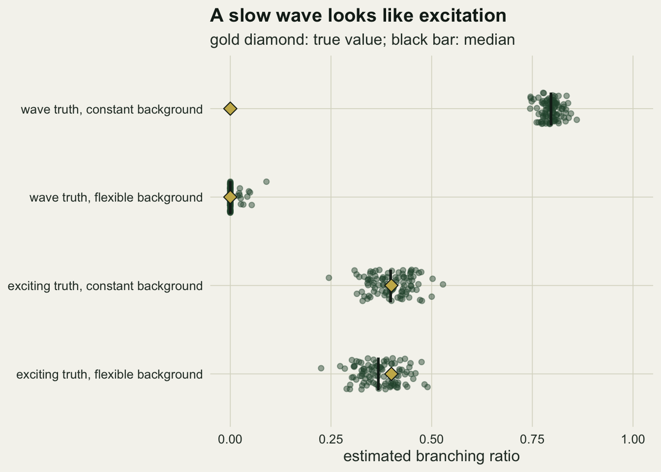
Excitation reads as a changing background
The reverse cross fit takes the self-exciting series and fits the same 16 term spline background with no excitation, the time analogue of fitting a smooth intensity surface to a clustered map. As a reference, the same spline is fitted to Poisson series with the same mean count and no structure of any kind, so the spline’s own noise is measured rather than assumed to be zero.
swing_q <- rbind(hwk = quantile(cross[, "swing_hwk"], c(0.25, 0.5, 0.75)),
                 poi = quantile(cross[, "swing_poi"], c(0.25, 0.5, 0.75)))
rej_bg_hwk <- mean(cross[, "lr_bg_hwk"] > lr_crit)
rej_bg_poi <- mean(cross[, "lr_bg_poi"] > lr_crit)
rej_hk_wav <- mean(cross[, "lr_hk_wav"] > lr_crit)
rej_hk_hwk <- mean(cross[, "lr_hk_hwk"] > lr_crit)
mcse_rate <- function(p) sqrt(p * (1 - p) / n_rep)
swing_hk_med <- median(cross[, "swing_hwk_hk"])
# spline noise with only as many events as the Hawkes background explains
set.seed(2415)
swing_mu0 <- replicate(n_rep, {
  f <- fit_pp(sim_hawkes(bg_flat(mu0), mu0, 0, beta_true), k_flex, FALSE)
  m <- exp(drop(f$bas$Xg %*% f$par)); max(m) / min(m) })
swing_mu0_med <- median(swing_mu0)
set.seed(2416)   # bootstrap standard errors of the two medians
boot_med_se <- function(x) sd(replicate(1000, median(sample(x, replace = TRUE))))
se_swing_hk <- boot_med_se(cross[, "swing_hwk_hk"]); se_swing_mu0 <- boot_med_se(swing_mu0)
On the Poisson series the fitted background has a median ratio of highest to lowest rate of 2.44, which is the spline following noise. On the self-exciting series the median is 4.00 (interquartile range 3.06 to 5.49) for a background that is perfectly flat. A likelihood ratio test of the spline against a constant rate, on 15 degrees of freedom at the five per cent level, rejects the constant rate in 88 per cent of self-exciting series and 8 per cent of Poisson series (Monte Carlo standard error at most 5.0 points, so the Poisson rate is compatible with the nominal five). The model without excitation finds good days and bad days that were never there, and a formal test that assumes independent events agrees with it.
The same test inside the Hawkes model is better behaved. Comparing the 16 term background with a constant one, both with excitation, rejects the constant background in 100 per cent of wave series and in 9 per cent of self-exciting series with a flat background. Once the kernel is in the model the clusters rarely count as evidence for a wave. The fitted background still wanders, though: its median swing on the self-exciting series is 3.39. The Poisson reference above has too many events to be the right yardstick, since the background of the Hawkes fit only has to explain the immigrant detections. Fitted to Poisson series at the background rate of 0.4, the same spline has a median swing of 2.75, so noise accounts for most of the wandering. The two medians differ by 0.64, against bootstrap standard errors of 0.18 and 0.12 from a hundred replicates each, which suggests that the spline also absorbs some of the excitation but does not measure how much.
f_bg_p <- fit_pp(tt_hwk_ex, k_flex, FALSE)
f_bg_h <- fit_pp(tt_hwk_ex, k_flex)
grid_mid <- (seq_len(n_grid) - 0.5) * T_end / n_grid
bg_df <- rbind(
  data.frame(time = grid_mid, rate = exp(drop(f_bg_p$bas$Xg %*% f_bg_p$par)),
             fit = "spline background, no excitation"),
  data.frame(time = grid_mid, rate = exp(drop(f_bg_h$bas$Xg %*% f_bg_h$par[1:k_flex])),
             fit = "spline background with excitation"))
ex_swing_p <- max(bg_df$rate[bg_df$fit == "spline background, no excitation"]) /
  min(bg_df$rate[bg_df$fit == "spline background, no excitation"])
ggplot(bg_df, aes(time, rate, colour = fit)) +
  geom_hline(yintercept = mu0, linetype = "dashed", colour = te_ink, linewidth = 0.6) +
  geom_line(linewidth = 0.9) +
  geom_rug(data = data.frame(time = tt_hwk_ex), aes(x = time), inherit.aes = FALSE,
           colour = te_body, alpha = 0.35, length = unit(0.04, "npc")) +
  scale_colour_manual(values = c(te_rust, te_forest), name = NULL) +
  labs(x = "hours since the recorder was deployed", y = "background, detections per hour",
       title = "Clusters turned into weather",
       subtitle = "dashed: the true background; ticks: detections") +
  theme_datasheet() +
  theme(legend.position = "bottom")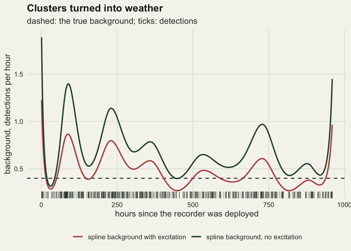
In this series the background fitted without excitation swings by a factor of 5.99, part of it from the spline flaring at the two ends of the window, and it runs above the true level for most of the forty days because it has to carry the provoked detections too. The background fitted with excitation sits lower and closer to the truth, but it follows the same bumps at a smaller size.
How flexible can the background be
A spline of 16 terms was a choice, and the two failures pull that choice in opposite directions. Too few terms and the wave leaks into the kernel; too many and the spline starts to follow the clusters. The sweep below refits both truths across basis sizes with 40 replicates per cell, a count fixed before running.
n_sweep <- 40
k_grid <- c(1, 4, 8, 12, 16, 24, 32)
set.seed(2413)
ks_rows <- lapply(k_grid, function(k) {
  e_wav <- replicate(n_sweep, fit_pp(sim_hawkes(bg_wave(P0), mu0 * exp(amp), 0, beta_true), k)$n_hat)
  e_hwk <- replicate(n_sweep, fit_pp(sim_hawkes(bg_flat(mu0), mu0, br_true, beta_true), k)$n_hat)
  data.frame(k = k, truth = c("wave, true n = 0", "self-exciting, true n = 0.4"),
             mean_n = c(mean(e_wav), mean(e_hwk)),
             se_n = c(sd(e_wav), sd(e_hwk)) / sqrt(n_sweep))
})
ksw <- do.call(rbind, ks_rows)
knot_gap <- function(k) T_end / (k - 3)
wav_at <- function(k) ksw$mean_n[ksw$k == k & ksw$truth == "wave, true n = 0"]
hwk_at <- function(k) ksw$mean_n[ksw$k == k & ksw$truth == "self-exciting, true n = 0.4"]
se_max <- max(ksw$se_n)ggplot(ksw, aes(k, mean_n, colour = truth)) +
geom_hline(yintercept = c(0, br_true), linetype = "dashed", colour = te_gold, linewidth = 0.7) +
geom_errorbar(aes(ymin = mean_n - 2 * se_n, ymax = mean_n + 2 * se_n), width = 0.8) +
geom_line(linewidth = 0.9) +
geom_point(size = 2.4) +
scale_colour_manual(values = c(te_forest, te_rust), name = NULL) +
scale_x_continuous(breaks = k_grid) +
labs(x = "spline terms in the background", y = "mean estimated branching ratio",
title = "A window, not a dial",
subtitle = "dashed gold: the two true values, 0 and 0.4") +
theme_datasheet() +
theme(legend.position = "bottom")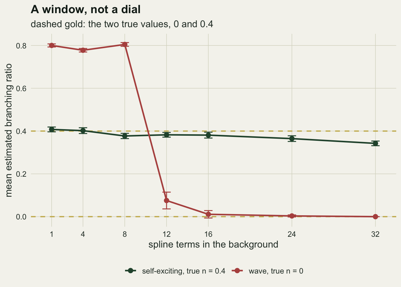
The wave truth needs enough terms to draw four cycles. At 8 terms the mean branching ratio of the wave series is still 0.805; at 12 it is 0.075, and from 16 terms on it is at most 0.011. The self-exciting truth loses excitation slowly as terms are added, from 0.408 with a constant background to 0.381 at 16 terms and 0.342 at 32. The largest Monte Carlo standard error in the sweep is 0.020. There is no basis size at which both truths are recovered without bias; there is a range where both errors are small, and its left edge is set by the background.
The separation depends on two time scales rather than on the basis size alone. The next sweep holds the basis at 16 terms, whose knots are 74 hours apart, and varies the period of the wave for the independent truth and the mean kernel delay 1 / beta for the self-exciting truth.
p_grid <- c(24, 48, 96, 240, 480)
d_grid <- c(0.5, 2, 8, 32)
set.seed(2414)
p_rows <- lapply(p_grid, function(P) {
  e <- replicate(n_sweep, fit_pp(sim_hawkes(bg_wave(P), mu0 * exp(amp), 0, beta_true), k_flex)$n_hat)
  data.frame(scale = P, mean_n = mean(e), se_n = sd(e) / sqrt(n_sweep))
})
d_rows <- lapply(d_grid, function(d) {
  e <- replicate(n_sweep, fit_pp(sim_hawkes(bg_flat(mu0), mu0, br_true, 1 / d), k_flex)$n_hat)
  data.frame(scale = d, mean_n = mean(e), se_n = sd(e) / sqrt(n_sweep))
})
psw <- do.call(rbind, p_rows); dsw <- do.call(rbind, d_rows)
gap_k <- knot_gap(k_flex)
p_wave <- ggplot(psw, aes(scale, mean_n)) +
geom_vline(xintercept = gap_k, linetype = "dotted", colour = te_body) +
geom_hline(yintercept = 0, linetype = "dashed", colour = te_gold, linewidth = 0.7) +
geom_errorbar(aes(ymin = mean_n - 2 * se_n, ymax = mean_n + 2 * se_n),
width = 0.06, colour = te_forest) +
geom_line(colour = te_forest, linewidth = 0.9) + geom_point(colour = te_forest, size = 2.4) +
scale_x_log10(breaks = p_grid) + coord_cartesian(ylim = c(0, 1)) +
labs(x = "background period, hours", y = "mean estimated branching ratio",
title = "No excitation, true n = 0") +
theme_datasheet()
p_delay <- ggplot(dsw, aes(scale, mean_n)) +
geom_vline(xintercept = gap_k, linetype = "dotted", colour = te_body) +
geom_hline(yintercept = br_true, linetype = "dashed", colour = te_gold, linewidth = 0.7) +
geom_errorbar(aes(ymin = mean_n - 2 * se_n, ymax = mean_n + 2 * se_n),
width = 0.06, colour = te_rust) +
geom_line(colour = te_rust, linewidth = 0.9) + geom_point(colour = te_rust, size = 2.4) +
scale_x_log10(breaks = c(d_grid, round(gap_k)), labels = c("0.5", "2", "8", "32", "74")) + coord_cartesian(ylim = c(0, 1)) +
labs(x = "mean kernel delay, hours", y = NULL,
title = "Self-exciting, true n = 0.4") +
theme_datasheet()
p_wave + p_delay +
plot_annotation(subtitle = "dotted: knot spacing of the sixteen term spline; dashed gold: truth",
theme = theme_datasheet())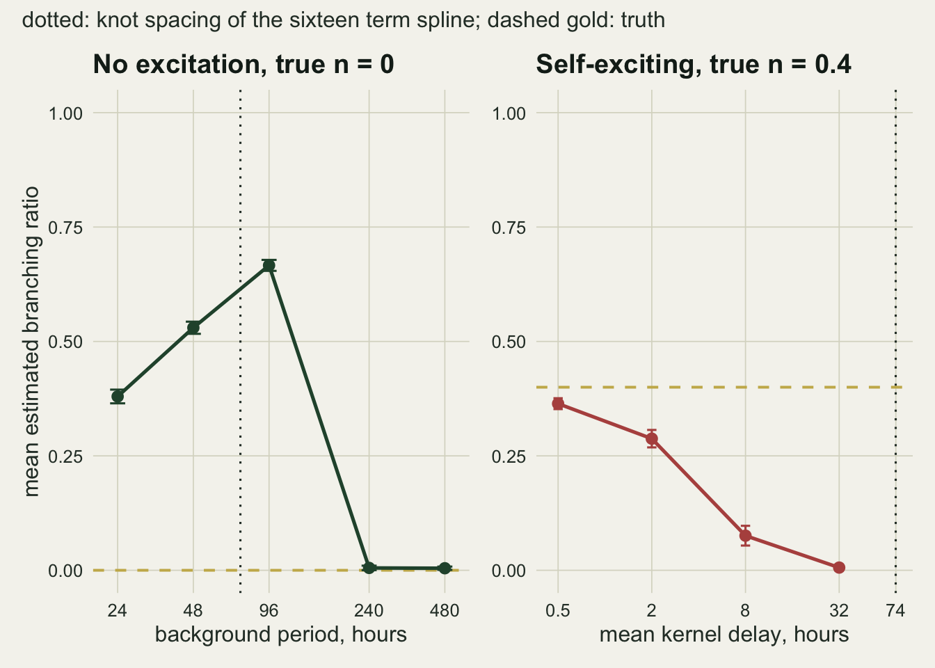
The wave panel is not monotone. A period of 24 hours, a daily rhythm, gives a mean branching ratio of 0.380; 48 hours gives 0.530, and 96 hours, just above the knot spacing, gives the worst value, 0.666. At 240 and 480 hours, several knot spacings per cycle, it is 0.005 and 0.004. A background that the spline cannot draw is read as excitation whatever its period, and the size of the error depends on how well a kernel can imitate the leftover wave.
The kernel panel is monotone and less forgiving than the basis sweep suggested. A mean delay of 0.5 hours, a 148th of the knot spacing, gives 0.364. A delay of 2 hours, a 37th of the knot spacing, already gives 0.288, a loss of 28 per cent of the true branching ratio; 8 hours gives 0.076, and 32 hours gives 0.006, with the excitation almost entirely inside the background. The flexible background separates the two stories only when the background changes over several knot spacings and the kernel fades within a very small part of one. As the two time scales approach each other, the confounding of the spatial case comes back well before they meet.
Residuals by time rescaling
The time rescaling theorem gives a residual check that needs no simulation; Ogata used it to check fitted earthquake sequences, and Brown and colleagues set it out as a goodness of fit test for point process models of spike trains. If the fitted conditional intensity is right, the compensator evaluated at the events turns them into a unit rate Poisson process, so the gaps between successive compensator values are independent standard exponentials. Two checks on the gaps follow: a Kolmogorov-Smirnov test of the gaps against the exponential, and the rank correlation between each gap and the next. A third check looks at slow variation instead: cut the rescaled time axis into blocks of equal length, count the events in each block, and compare the spread of the counts with the Poisson variance by a dispersion chi squared test. The block length changes what that test can see, so it was run at 20, 40 and 80 rescaled units, a set fixed before running. All three checks were computed for the fits of the cross simulation, including the correct constant background Hawkes fit to the self-exciting series as a reference.
rs <- function(tag) c(ks_rej = mean(cross[, paste0(tag, ".ks")] < 0.05),
                      ac_mean = mean(cross[, paste0(tag, ".ac")]),
                      ac_se = sd(cross[, paste0(tag, ".ac")]) / sqrt(n_rep),
                      d20_rej = mean(cross[, paste0(tag, ".d20")] < 0.05),
                      d40_rej = mean(cross[, paste0(tag, ".d40")] < 0.05),
                      d80_rej = mean(cross[, paste0(tag, ".d80")] < 0.05))
res_tab <- rbind(wav_h1 = rs("r_wav_h1"), wav_hk = rs("r_wav_hk"),
                 hwk_pk = rs("r_hwk_pk"), hwk_hk = rs("r_hwk_hk"),
                 hwk_h1 = rs("r_hwk_h1"))
round(res_tab, 3)
ks_rej ac_mean ac_se d20_rej d40_rej d80_rej
wav_h1 0.01 -0.009 0.004 0.06 0.45 0.00
wav_hk 0.02 -0.028 0.004 0.00 0.00 0.00
hwk_pk 1.00 0.145 0.004 0.57 0.09 0.00
hwk_hk 0.00 0.000 0.003 0.01 0.00 0.00
hwk_h1 0.00 -0.002 0.003 0.03 0.04 0.05The gap checks catch missing excitation without fail. When the self-exciting series are fitted with a spline background and no kernel, the Kolmogorov-Smirnov test rejects in 100 per cent of replicates, and consecutive rescaled gaps have a mean rank correlation of 0.145, because a short gap inside a cluster is followed by another short gap. The Hawkes fit with a flexible background on the same series rejects in 0 per cent, with a gap correlation of 0.000.
Neither of these two gap-based checks catches the other mistake. The constant background Hawkes fit to the wave series, the one that reported a branching ratio near 0.80 for a process with none, is rejected by the Kolmogorov-Smirnov test in 1 per cent of replicates, and its gap correlation is -0.009 (standard error 0.004); for comparison the flexible fit to the same series gives -0.028, so this statistic has no reference at zero here either. The correct fits are rejected by the Kolmogorov-Smirnov test in 2, 0 and 0 per cent of replicates, so the wrong model is not rejected more often than the right ones. That is not the conservativeness of a test with estimated parameters, measured in testing a fitted distribution; it is lack of power. The intensity of the wrong model jumps after each detection and follows the good days closely enough that the gaps between consecutive events carry almost no information about a rate change over days.
The block counts do carry it. In blocks of 40 rescaled units the dispersion test rejects the wrong model in 45 per cent of wave series and the correct constant background fit in 4 per cent of self-exciting series (Monte Carlo standard error at most 5.0 points). The block length matters: in blocks of 20 units the rates are 6 and 3 per cent, and in blocks of 80 units they are 0 and 5 per cent. Short blocks have little power against the wave and also react to unmodelled clusters: in blocks of 20 units the test rejects the spline fit without excitation on the self-exciting series in 57 per cent. Long blocks average the wave out. Without knowing the time scale of the background there is no principled way to pick the length.
So the answer to the spatial warning is partial. Time makes the confounding measurable in one direction by the gap residuals. In the other the gap residuals see nothing, and the evidence has to come from a likelihood ratio between background models fitted with the kernel included, or from a residual aimed at slow variation, whose power depends on a block length matched to the background.
What to report
Report the branching ratio, not alpha or beta alone, together with the background model it was estimated under. In the constant background fits the ratio had a smaller coefficient of variation than the kick size, and the kick size and decay rate moved together. When the branching ratio is estimated at or near zero, do not print a decay rate beside it: the likelihood is flat in beta there, and the fitted value is whatever the optimiser stopped at.
Fit the Hawkes model with more than one background, and show the branching ratio across them. A single fit with a constant background says nothing about excitation when the recording spans weather, season or daylight, because a background wave alone produced a branching ratio near four fifths here. The basis sweep is the evidence to show, but a collapse of the branching ratio as the background becomes flexible does not by itself say which story is true. A self-exciting process whose kernel lasts hours rather than minutes also loses most of its branching ratio: 0.076 at a delay of 8 hours with 16 terms, for a true 0.4. The kernel delay cannot be read from the flexible fits once the ratio is near zero, so it has to come from the simple background fit, and there the wave series of this post gave a spurious kernel with a mean delay of 9.8 hours, shorter than the knot spacing by a factor of 8 but longer than the 8 hour kernel that also collapsed. In this post’s own example, then, the collapse was not evidence against excitation: a real kernel of that length would also have lost most of its branching ratio. A collapse can only point to the background when the delay fitted under the simple background is a very small fraction of the knot spacing, as the true half hour kernel was when it kept most of its ratio, and a fitted delay of several hours is itself a warning that the kernel may be imitating the background. Outside that case the decision needs knowledge from outside the event series, such as how quickly a real response to a call can follow it, or a measured driver of the background.
Give the time scales. State the mean kernel delay, the spacing of the background knots and any known periodic driver, such as the daily cycle. The separation worked when the background changed over several knot spacings and the kernel decayed within a very small part of one; a kernel delay of a 37th of the knot spacing already lost 28 per cent of the branching ratio.
Use the gap residuals from time rescaling to look for missing excitation, and a likelihood ratio between background models fitted with the kernel included to look for a missing background, with block counts of the rescaled events as a second, weaker check. The gap residuals passed a model that invented four fifths of the events as offspring.
Honest limits
Every simulated background here is a single sine wave on the log scale, with a period fixed in advance, and every kernel is exponential. Real calling activity has a daily rhythm, weather that arrives irregularly and a season, and a real counter-singing response may peak after a delay rather than immediately. A kernel of the wrong shape changes the estimated branching ratio, and nothing above measures by how much. The delay of the spurious kernel fitted to the wave was recorded for one wave only, at one period and amplitude, so how slow a spurious kernel comes out for other backgrounds is not known from this post.
The flexible background is an unpenalised B-spline whose size was chosen by sweeping, with the truth known. On real data the truth is not known, and choosing the basis size by an information criterion or a penalty would need its own simulation at the time scales of the data in hand. The daily wave was read as excitation at sixteen terms; a basis with a daily periodic term would handle it, but only because the period is known in advance.
The likelihood ratio tests of the background use the chi squared reference on fifteen degrees of freedom. Under the null that was simulated, a flat self-exciting series, the branching ratio lies well inside its range (from 0.226 to 0.490 in the flexible fits), so the reference is the usual large-sample one; but sixteen unpenalised spline terms on a few hundred events is not a large sample, and the rejection rates under true nulls came out at 9 per cent for the Hawkes comparison on flat self-exciting series and 8 per cent for the comparison without excitation on Poisson series. Both are above the nominal five but within two Monte Carlo standard errors of it (one standard error is 2.2 points at a true rate of five per cent), so a hundred replicates can neither show nor exclude a small excess. If the null truth had no excitation, the branching ratio would sit on its lower bound and the decay rate would be undefined, and the usual reference would lose its justification. The dispersion test of the block counts also treats the fitted compensator as known, and that matters: on the correct fits with a sixteen term background it rejected in 0 per cent of wave series and 0 per cent of self-exciting series in blocks of 40 units, because the spline absorbs the variation between blocks. Its chi squared reference is only usable for a background with few terms. A parametric bootstrap would calibrate these tests, and none was run.
A detection is not a call. A recorder misses quiet calls, and a detector that fires twice on one call manufactures an offspring event with a very short delay. Both change the apparent excitation, and a real analysis would need a lower bound on the delay or an explicit detection model.
The model is univariate. When two birds answer each other, the natural model has two streams and a cross-excitation kernel from each to the other, and when several recorders share weather, a background shared among recorders is the better way to absorb the good days. Neither extension is shown.
References
Hawkes AG 1971 Biometrika 58(1):83-90 (10.1093/biomet/58.1.83)
Ozaki T 1979 Annals of the Institute of Statistical Mathematics 31(1):145-155 (10.1007/BF02480272)
Ogata Y 1981 IEEE Transactions on Information Theory 27(1):23-31 (10.1109/TIT.1981.1056305)
Ogata Y 1988 Journal of the American Statistical Association 83(401):9-27 (10.1080/01621459.1988.10478560)
Brown EN, Barbieri R, Ventura V, Kass RE, Frank LM 2002 Neural Computation 14(2):325-346 (10.1162/08997660252741149)