library(ggplot2)
library(grid)

te_pal <- list(forest = "#275139", green = "#2f8f63", sage = "#93a87f",
               clay = "#b5534e", gold = "#cda23f", line = "#dad9ca",
               ink = "#16241d", paper = "#f5f4ee")

theme_te <- function() {
  theme_minimal(base_size = 12) +
    theme(panel.grid.minor = element_blank(),
          panel.grid.major = element_line(colour = "#e7e6dc"),
          plot.background = element_rect(fill = "#f5f4ee", colour = NA),
          panel.background = element_rect(fill = "#f5f4ee", colour = NA),
          plot.title = element_text(face = "bold", colour = te_pal$ink),
          axis.title = element_text(colour = "#2c3a31"))
}Reintroduction release strategies
R
conservation
reintroduction
PVA
population dynamics
ecology tutorial
ggplot2
Release size, schedule and stage composition compared in R against a stochastic Lefkovitch model, with post-release mortality and a measured stopping rule.
A reintroduction programme almost never gets to choose how many animals it has. The donor population, the captive facility or the permit decides that, and the number arrives as a constraint. What the programme does choose is how to spend it: all in one year or a few animals a year for a decade, all adults or mostly juveniles, one site or several. Those choices are usually made on husbandry grounds and then defended after the fact with a population model. It is worth running the model first, because the choices are not equivalent and the differences are large enough to decide whether the release succeeds.
This post treats the release as a small optimisation problem. The objective is establishment: the population being above a stated size at a stated horizon. The decision variables are the total number released, the number of years over which it is spread, and the fraction of the released animals that are adults. The constraint is the total. Everything is measured against a three-stage matrix model projected with demographic stochasticity, plus a post-release survival penalty applied in the settling year, because animals that have just been moved do not survive like residents.
Two earlier posts are the groundwork. Stage-structured Lefkovitch matrices in R builds the projection matrix and explains the eigenvalue, the stable stage distribution and the reproductive values, all of which are used here without re-deriving them. Allee effects and extinction risk explains why small introductions fail more often than a deterministic growth rate suggests. This post is about allocation, not about the Allee threshold: there is no mate-finding term in the model below, and the failure of small releases here comes from demographic stochasticity alone.
The population and its matrix
Three stages: juvenile, subadult, adult. Juveniles survive one year and all of the survivors become subadults. Subadults survive and then either stay subadult or move up. Adults survive and breed. That is a Lefkovitch matrix, built by hand, with a post-breeding annual census.
fec <- 0.80; s_j <- 0.52; s_s <- 0.68; gam <- 0.80; s_a <- 0.80

make_A <- function(fecundity) matrix(
  c(0, 0, fecundity,
    s_j, s_s * (1 - gam), 0,
    0, s_s * gam, s_a),
  nrow = 3, byrow = TRUE,
  dimnames = list(c("juvenile", "subadult", "adult"),
                  c("juvenile", "subadult", "adult")))

A <- make_A(fec)
print(A)
juvenile subadult adult
juvenile 0.00 0.000 0.8
subadult 0.52 0.136 0.0
adult 0.00 0.544 0.8ev <- eigen(A)
lambda <- Re(ev$values[1])
w <- Re(ev$vectors[, 1]); w <- w / sum(w)
v <- Re(eigen(t(A))$vectors[, 1]); v <- v / v[1]
print(round(c(lambda = lambda, stable_juv = w[1], stable_sub = w[2],
stable_ad = w[3]), 4)) lambda stable_juv stable_sub stable_ad
1.0405 0.3478 0.1999 0.4523 print(round(c(rv_juvenile = v[1], rv_subadult = v[2], rv_adult = v[3],
rv_ratio_juv_over_ad = v[1] / v[3]), 4)) rv_juvenile rv_subadult rv_adult
1.0000 2.0009 3.3268
rv_ratio_juv_over_ad
0.3006 The dominant eigenvalue is 1.0405, so a population already at its stable stage distribution grows by about four per cent a year once it is large enough for the averages to hold. The stable stage distribution is 0.3478 juveniles, 0.1999 subadults and 0.4523 adults. The left eigenvector gives the reproductive values, scaled so a juvenile is worth one: a subadult is worth 2.0009 juveniles and an adult is worth 3.3268. Equivalently, one juvenile is worth 0.3006 of an adult. That last number will come back as the answer to the composition question, which is not obvious yet.
Two definitions have to be stated before anything is optimised, because establishment is not a property of a population, it is a property of a criterion. Here a release has established if the population is at or above 100 individuals at year 25. Both numbers are choices. A lower threshold makes every strategy look better, and so does a longer horizon, because the growth rate here is above one and time therefore works for any founder group that gets through its release years. Move either number and the strategies do not simply shift together: the gaps between them change as well.
nyr <- 25; thresh <- 100; p_bad <- 0.15; bad_mult <- 0.20
print(c(horizon_years = nyr, establishment_threshold = thresh,
        bad_release_year_prob = p_bad, bad_year_multiplier = bad_mult))
horizon_years establishment_threshold bad_release_year_prob
25.00 100.00 0.15
bad_year_multiplier
0.20 The last two constants describe release-year quality. In any given year the released animals meet whatever weather, food supply and predator pressure that year happens to have, and all of the animals released in that year meet the same conditions. With probability 0.15 a release year is bad and post-release survival in that year is multiplied by 0.20. This is the only correlated risk in the model, and it is what makes the schedule question interesting rather than arithmetic.
The projection engine
Demographic stochasticity is put in the obvious way: survival is binomial with the matrix entry as the probability, and recruitment is Poisson with the fecundity times the number of adults as the mean. The transition out of the subadult stage is a second binomial applied to the survivors, which reproduces the stasis and advancement entries exactly.
The whole thing is vectorised over replicates. The state is three integer vectors of length equal to the number of replicates, and rbinom and rpois are both vectorised over their size and rate arguments, so one call advances every replicate at once. The loop runs over years, of which there are 25, rather than over replicates, of which there are up to 20000. Written the other way this post would take a quarter of an hour instead of a quarter of a minute.
Released animals are thinned once, at release, by a stage-specific post-release survival. This is the settling penalty: only a fraction of the animals put out survive the disruption of being moved, and they suffer resident mortality on top of that in the same year. Released juveniles enter the juvenile stage and released adults enter the adult stage.
allocate <- function(total, nrel) {
  base <- total %/% nrel; extra <- total %% nrel
  base + c(rep(1L, extra), rep(0L, nrel - extra))
}

run_release <- function(total, nrel, adult_frac, phi_j, phi_a, nrep,
                        fecundity = fec, seed = 20260719, years = nyr,
                        check = years, keep = FALSE) {
  set.seed(seed)
  al <- allocate(total, nrel)
  Nj <- Ns <- Na <- integer(nrep)
  settled <- integer(nrep)
  traj <- if (keep) matrix(0L, years + 1L, nrep) else NULL
  hits <- numeric(0)
  for (t in seq_len(years)) {
    if (t <= nrel) {
      n_ad <- round(al[t] * adult_frac); n_jv <- al[t] - n_ad
      qual <- ifelse(rbinom(nrep, 1, p_bad) == 1, bad_mult, 1)
      got_j <- rbinom(nrep, n_jv, pmin(phi_j * qual, 1))
      got_a <- rbinom(nrep, n_ad, pmin(phi_a * qual, 1))
      Nj <- Nj + got_j; Na <- Na + got_a
      settled <- settled + got_j + got_a
    }
    if (keep) traj[t, ] <- Nj + Ns + Na
    rec  <- rpois(nrep, fecundity * Na)
    sv_j <- rbinom(nrep, Nj, s_j)
    sv_s <- rbinom(nrep, Ns, s_s)
    adv  <- rbinom(nrep, sv_s, gam)
    sv_a <- rbinom(nrep, Na, s_a)
    Nj <- rec; Ns <- sv_j + (sv_s - adv); Na <- adv + sv_a
    if (t %in% check) hits <- c(hits, mean((Nj + Ns + Na) >= thresh))
  }
  tot <- Nj + Ns + Na
  if (keep) traj[years + 1L, ] <- tot
  list(p_est = hits, p_wipe = mean(settled < 0.25 * total),
       mean_cond = if (any(tot >= thresh)) mean(tot[tot >= thresh]) else NA_real_,
       traj = traj)
}
Every call sets the same seed before it starts, so two strategies compared with each other see the same random number stream. That is common random numbers, and it makes a sweep across a decision variable far smoother than independent replicates would, because most of the difference between two neighbouring settings is real rather than sampling noise.
Does the simulation reproduce the matrix
A stochastic projection is only trustworthy if it reproduces the deterministic model when the stochasticity is made irrelevant. Start a large population at the stable stage distribution, run it forward with no releases and no post-release penalty, and the mean log growth rate should match the log of the dominant eigenvalue.
verify_growth <- function(nrep, years, n0, fecundity = fec, seed = 4711) {
  set.seed(seed)
  start <- round(n0 * w)
  Nj <- rep(start[1], nrep); Ns <- rep(start[2], nrep); Na <- rep(start[3], nrep)
  n_start <- Nj + Ns + Na
  for (t in seq_len(years)) {
    rec  <- rpois(nrep, fecundity * Na)
    sv_j <- rbinom(nrep, Nj, s_j)
    sv_s <- rbinom(nrep, Ns, s_s)
    adv  <- rbinom(nrep, sv_s, gam)
    sv_a <- rbinom(nrep, Na, s_a)
    Nj <- rec; Ns <- sv_j + (sv_s - adv); Na <- adv + sv_a
  }
  tot <- Nj + Ns + Na
  c(sim_log_growth = mean(log(tot / n_start)) / years,
    final_juv_share = mean(Nj / tot), final_sub_share = mean(Ns / tot),
    final_ad_share = mean(Na / tot))
}

nrep_check <- 600; years_check <- 30; n0_check <- 4000
vg <- verify_growth(nrep_check, years_check, n0_check)
print(c(replicates = nrep_check, years = years_check, start_N = n0_check))
replicates years start_N
600 30 4000 print(round(c(det_log_lambda = log(lambda), vg[1],
discrepancy = vg[1] - log(lambda),
implied_lambda = exp(vg[1])), 5)) det_log_lambda sim_log_growth
0.03968 0.03963
discrepancy.sim_log_growth implied_lambda.sim_log_growth
-0.00004 1.04043 print(round(c(vg[2:4], stable_juv = w[1], stable_sub = w[2],
stable_ad = w[3]), 4))final_juv_share final_sub_share final_ad_share stable_juv stable_sub
0.3477 0.1999 0.4524 0.3478 0.1999
stable_ad
0.4523 Over 600 replicates of 30 years starting from 4000 animals, the simulated mean log growth rate is 0.03963 against a deterministic 0.03968, a discrepancy of -0.00004, which corresponds to an implied growth rate of 1.04043 against the eigenvalue of 1.0405. The stage shares after 30 years are 0.3477, 0.1999 and 0.4524, matching the stable distribution to three decimal places. The machinery is doing what the matrix says.
The small negative discrepancy is not a bug and it does not go away with more replicates. The mean of a log is below the log of a mean, so demographic stochasticity depresses the average log growth rate even when it leaves the expected population size untouched. At 4000 animals the effect is in the fifth decimal place. At 40 animals, which is where a reintroduction actually starts, it is the whole problem.
One release or several
Fix the total at 120 animals, half of them adults, with a post-release survival of 0.6 for both stages, and vary only the number of years the release is spread over. Compare one year, two, five and ten. Two other quantities are recorded alongside establishment probability, because they are the two competing mechanisms and they pull in opposite directions.
The first is founder wipe-out: the probability that fewer than a quarter of the released animals survive their settling year. With a post-release survival of 0.6 that only happens when a large share of the animals met a bad release year. The second is the mean population size at the horizon among the replicates that did establish, which measures how much room a strategy leaves above the threshold rather than how often it clears it.
phi_base <- 0.60
sched <- c(1, 2, 5, 10)
nrep_sched <- 20000

tab_sched <- do.call(rbind, lapply(sched, function(k) {
  a <- run_release(120, k, 0.5, phi_base, phi_base, nrep_sched)
  b <- run_release(60, k, 0.5, phi_base, phi_base, nrep_sched)
  data.frame(release_years = k, p_est_120 = a$p_est, p_est_60 = b$p_est,
             p_wipeout = a$p_wipe, mean_N_given_est = a$mean_cond)
}))

print(c(replicates = nrep_sched, base_total = 120, small_total = 60,
        post_release_survival = phi_base))
replicates base_total small_total
20000.0 120.0 60.0
post_release_survival
0.6 print(round(tab_sched, 4)) release_years p_est_120 p_est_60 p_wipeout mean_N_given_est
1 1 0.8125 0.3370 0.1523 190.5685
2 2 0.8243 0.2984 0.0232 179.8158
3 5 0.8384 0.2364 0.0024 166.1285
4 10 0.7907 0.1573 0.0000 152.4046print(round(c(spread_120 = max(tab_sched$p_est_120) - min(tab_sched$p_est_120),
best_sched_120 = tab_sched$release_years[which.max(tab_sched$p_est_120)],
spread_60 = max(tab_sched$p_est_60) - min(tab_sched$p_est_60),
best_sched_60 = tab_sched$release_years[which.max(tab_sched$p_est_60)],
wipe_ratio = tab_sched$p_wipeout[1] / tab_sched$p_wipeout[3],
meanN_drop_pct = 100 *
(1 - tab_sched$mean_N_given_est[4] / tab_sched$mean_N_given_est[1])), 4)) spread_120 best_sched_120 spread_60 best_sched_60 wipe_ratio
0.0478 5.0000 0.1798 1.0000 63.4583
meanN_drop_pct
20.0264 n_show <- 120
tr1 <- run_release(120, 1, 0.5, phi_base, phi_base, n_show, keep = TRUE)$traj
tr5 <- run_release(120, 5, 0.5, phi_base, phi_base, n_show, keep = TRUE)$traj
pack <- function(m, lab) {
data.frame(year = rep(seq_len(nrow(m)) - 1L, times = ncol(m)),
N = as.vector(m),
rep = rep(seq_len(ncol(m)), each = nrow(m)),
sched = lab)
}
traj_long <- rbind(pack(tr1, "All 120 in one year"),
pack(tr5, "24 a year for five years"))
traj_long$N[traj_long$N < 1] <- 0.6
final <- traj_long[traj_long$year == nyr, c("rep", "sched", "N")]
names(final)[3] <- "final_N"
traj_long <- merge(traj_long, final, by = c("rep", "sched"))
traj_long$outcome <- ifelse(traj_long$final_N >= thresh, "established", "failed")
traj_long$sched <- factor(traj_long$sched,
levels = c("All 120 in one year", "24 a year for five years"))
ggplot(traj_long, aes(year, N, group = interaction(rep, sched), colour = outcome)) +
geom_hline(yintercept = thresh, colour = te_pal$gold, linewidth = 0.7,
linetype = "22") +
geom_line(linewidth = 0.28, alpha = 0.55) +
facet_wrap(~sched) +
scale_y_log10() +
scale_colour_manual(values = c(established = te_pal$forest,
failed = te_pal$clay), name = NULL) +
labs(x = "Year", y = "Population size",
title = "Two ways to spend the same 120 animals") +
theme_te() +
theme(legend.position = "top",
strip.text = element_text(colour = te_pal$ink, face = "bold"))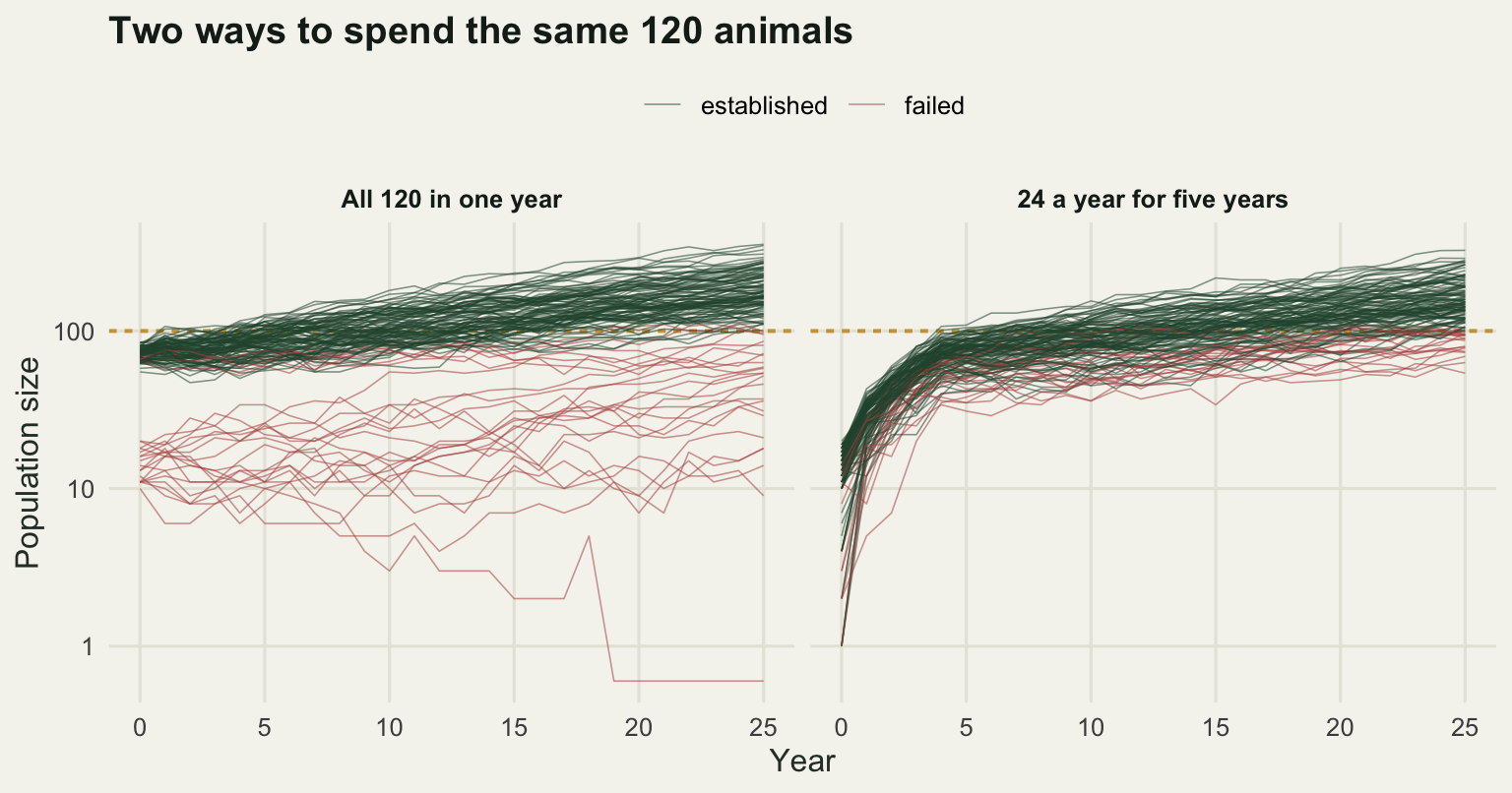
mech <- rbind(
  data.frame(release_years = tab_sched$release_years, value = tab_sched$p_est_120,
             panel = "Establishment probability"),
  data.frame(release_years = tab_sched$release_years, value = tab_sched$p_wipeout,
             panel = "Founder wipe-out probability"),
  data.frame(release_years = tab_sched$release_years,
             value = tab_sched$mean_N_given_est,
             panel = "Mean N at year 25 given establishment"))
mech$panel <- factor(mech$panel, levels = c(
  "Establishment probability", "Founder wipe-out probability",
  "Mean N at year 25 given establishment"))

ggplot(mech, aes(release_years, value)) +
  geom_line(colour = te_pal$forest, linewidth = 0.8) +
  geom_point(colour = te_pal$clay, size = 2.4) +
  facet_wrap(~panel, ncol = 1, scales = "free_y") +
  scale_x_continuous(breaks = sched) +
  labs(x = "Number of release years", y = NULL,
       title = "The schedule trades two risks against each other") +
  theme_te() +
  theme(strip.text = element_text(colour = te_pal$ink, face = "bold"))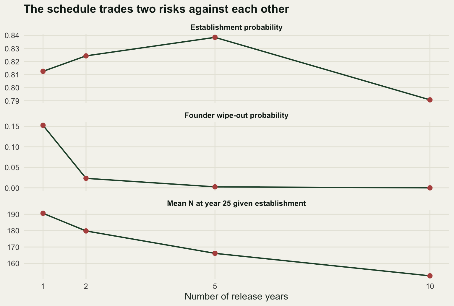
At a total of 120 the establishment probabilities are 0.8125 for a single release, 0.8243 over two years, 0.8384 over five and 0.7907 over ten. The optimum is interior, at five years, and the whole spread across the four schedules is 0.0478. That is a real difference at 20000 replicates but it is much smaller than the difference between having 100 animals and having 120, which the section on the marginal animal prices.
The two mechanisms are both large and they nearly cancel. Founder wipe-out is 0.1523 under a single release and 0.0024 when the release is spread over five years, a factor of 63.4583. That is straightforward: a one-off release stakes the entire founder group on one year’s conditions, and one year in about seven is bad. Spreading buys insurance against that, and the insurance is close to complete by five years.
Working the other way, the mean population at the horizon among successful runs falls from 190.5685 under a single release to 152.4046 over ten years, a drop of 20.0264 per cent. Animals released in year 10 have fifteen years of compounding left, not twenty-five. A spread release that establishes does so with less margin above the threshold, and if the threshold were higher the ranking would move.
There is a third thing in the table that I did not expect, and it is the more useful result. At a total of 60 rather than 120, spreading stops helping and starts hurting: 0.3370 for a single release falling monotonically to 0.1573 over ten years, a spread of 0.1798, which is nearly four times the spread at 120 animals. When the total is small enough that the founder group is genuinely at risk of demographic extinction, spreading it out is actively harmful, because it means the population spends its most fragile years even smaller than it needed to. Insurance against a bad release year is worth nothing if the uninsured part of the population dies of bad luck first. The advice “spread your releases” is therefore conditional on the total, and the condition is exactly the one a struggling programme fails.
Who to release
Now hold the total at 120 and the schedule at five years, and sweep the fraction of adults from zero to one, with the remainder made up of juveniles. Do it twice. First with equal post-release survival of 0.6 for both stages, which is the assumption a model makes when nobody has measured otherwise. Then with adults penalised to 0.15, a quarter of the juvenile value, which is what happens when translocated adults have a settled home range somewhere else, walk out of the release area looking for it, and never come back.
af_grid <- seq(0, 1, by = 0.125)
nrep_comp <- 8000
phi_a_pen <- 0.15

comp <- data.frame(
  adult_frac = af_grid,
  equal = sapply(af_grid, function(f)
    run_release(120, 5, f, phi_base, phi_base, nrep_comp)$p_est),
  penalised = sapply(af_grid, function(f)
    run_release(120, 5, f, phi_base, phi_a_pen, nrep_comp)$p_est))

print(c(replicates = nrep_comp, adult_phi_penalised = phi_a_pen,
        ratio_penalised = phi_a_pen / phi_base))
replicates adult_phi_penalised ratio_penalised
8000.00 0.15 0.25 print(round(comp, 4)) adult_frac equal penalised
1 0.000 0.1814 0.1814
2 0.125 0.3718 0.1746
3 0.250 0.5688 0.1709
4 0.375 0.7265 0.1629
5 0.500 0.8408 0.1476
6 0.625 0.9067 0.1325
7 0.750 0.9469 0.1281
8 0.875 0.9676 0.1150
9 1.000 0.9835 0.1138print(round(c(best_af_equal = comp$adult_frac[which.max(comp$equal)],
best_p_equal = max(comp$equal),
best_af_penalised = comp$adult_frac[which.max(comp$penalised)],
best_p_penalised = max(comp$penalised),
equal_all_adult_over_all_juv = comp$equal[9] / comp$equal[1],
pen_all_juv_over_all_adult = comp$penalised[1] / comp$penalised[9]), 4)) best_af_equal best_p_equal
1.0000 0.9835
best_af_penalised best_p_penalised
0.0000 0.1814
equal_all_adult_over_all_juv pen_all_juv_over_all_adult
5.4225 1.5945 With equal post-release survival the answer is as adult-heavy as possible. The optimum is an adult fraction of 1 with an establishment probability of 0.9835, against 0.1814 for an all juvenile release of the same 120 animals: a factor of 5.4225 from a decision that costs nothing. Adults breed immediately and survive at 0.8 a year, whereas a juvenile has to survive at 0.52 and then pass through the subadult stage before it contributes anything. The reproductive values already said this. An adult is worth 3.3268 juveniles, and the establishment probability follows the reproductive value of the released group rather than its head count.
With adults penalised to 0.15 the whole sweep inverts. The optimum is an adult fraction of 0 with an establishment probability of 0.1814, and an all adult release now manages only 0.1138, so juveniles win by a factor of 1.5945. The best available strategy under the penalty is no better than the worst available strategy without it: both are the all juvenile release at 0.1814, because that is the one strategy the penalty cannot touch. That is the honest way to describe what post-release dispersal costs.
Where the ranking flips
The two regimes above are two points on a continuum. The quantity that matters is the ratio of adult to juvenile post-release survival, and there is a value of that ratio at which the two extreme compositions are exactly equal. Sweep it and interpolate.
rho_grid <- c(0.20, 0.25, 0.28, 0.30, 0.32, 0.34, 0.40, 0.50)
nrep_cross <- 12000

cross <- data.frame(
  ratio = rho_grid,
  all_adult = sapply(rho_grid, function(r)
    run_release(120, 5, 1, phi_base, phi_base * r, nrep_cross)$p_est),
  all_juv = sapply(rho_grid, function(r)
    run_release(120, 5, 0, phi_base, phi_base * r, nrep_cross)$p_est))
cross$diff <- cross$all_adult - cross$all_juv

print(c(replicates = nrep_cross))
replicates
12000 print(round(cross, 4)) ratio all_adult all_juv diff
1 0.20 0.0526 0.1927 -0.1401
2 0.25 0.1113 0.1927 -0.0813
3 0.28 0.1585 0.1927 -0.0342
4 0.30 0.1963 0.1927 0.0037
5 0.32 0.2304 0.1927 0.0377
6 0.34 0.2726 0.1927 0.0799
7 0.40 0.4098 0.1927 0.2171
8 0.50 0.6106 0.1927 0.4179rho_star <- approx(cross$diff, cross$ratio, xout = 0)$y
print(round(c(measured_crossover = rho_star,
predicted_from_reproductive_value = v[1] / v[3],
difference = rho_star - v[1] / v[3],
mc_se_at_p_half = sqrt(0.25 / nrep_cross)), 4)) measured_crossover predicted_from_reproductive_value
0.2981 0.3006
difference mc_se_at_p_half
-0.0025 0.0046 comp_long <- rbind(
data.frame(x = comp$adult_frac, y = comp$equal,
series = "Equal post-release survival"),
data.frame(x = comp$adult_frac, y = comp$penalised,
series = "Adults at a quarter of juvenile survival"))
p_left <- ggplot(comp_long, aes(x, y, colour = series)) +
geom_line(linewidth = 0.9) +
geom_point(size = 1.9) +
scale_colour_manual(values = c(te_pal$clay, te_pal$forest), name = NULL) +
coord_cartesian(ylim = c(0, 1)) +
labs(x = "Fraction of released animals that are adults",
y = "Establishment probability",
title = "Establishment against release composition") +
theme_te() +
theme(legend.position = "top", legend.direction = "vertical",
plot.title = element_text(face = "bold", size = 11.5,
colour = te_pal$ink))
cross_long <- rbind(
data.frame(x = cross$ratio, y = cross$all_adult, series = "All adults"),
data.frame(x = cross$ratio, y = cross$all_juv, series = "All juveniles"))
p_right <- ggplot(cross_long, aes(x, y, colour = series)) +
geom_vline(xintercept = rho_star, colour = te_pal$gold, linewidth = 0.7,
linetype = "22") +
geom_line(linewidth = 0.9) +
geom_point(size = 1.9) +
scale_colour_manual(values = c(te_pal$forest, te_pal$clay), name = NULL) +
labs(x = "Ratio of adult to juvenile post-release survival",
y = "Establishment probability",
title = "Where the two extreme compositions cross") +
theme_te() +
theme(legend.position = "top", legend.direction = "vertical",
plot.title = element_text(face = "bold", size = 11.5,
colour = te_pal$ink))
grid.newpage()
grid.rect(gp = gpar(fill = te_pal$paper, col = NA))
pushViewport(viewport(layout = grid.layout(2, 2,
heights = unit(c(2.2, 1),
c("lines", "null")))))
grid.text("Which stage to release depends on the post-release survival ratio",
vp = viewport(layout.pos.row = 1, layout.pos.col = 1:2),
gp = gpar(fontface = "bold", fontsize = 14, col = te_pal$ink))
print(p_left, vp = viewport(layout.pos.row = 2, layout.pos.col = 1))
print(p_right, vp = viewport(layout.pos.row = 2, layout.pos.col = 2))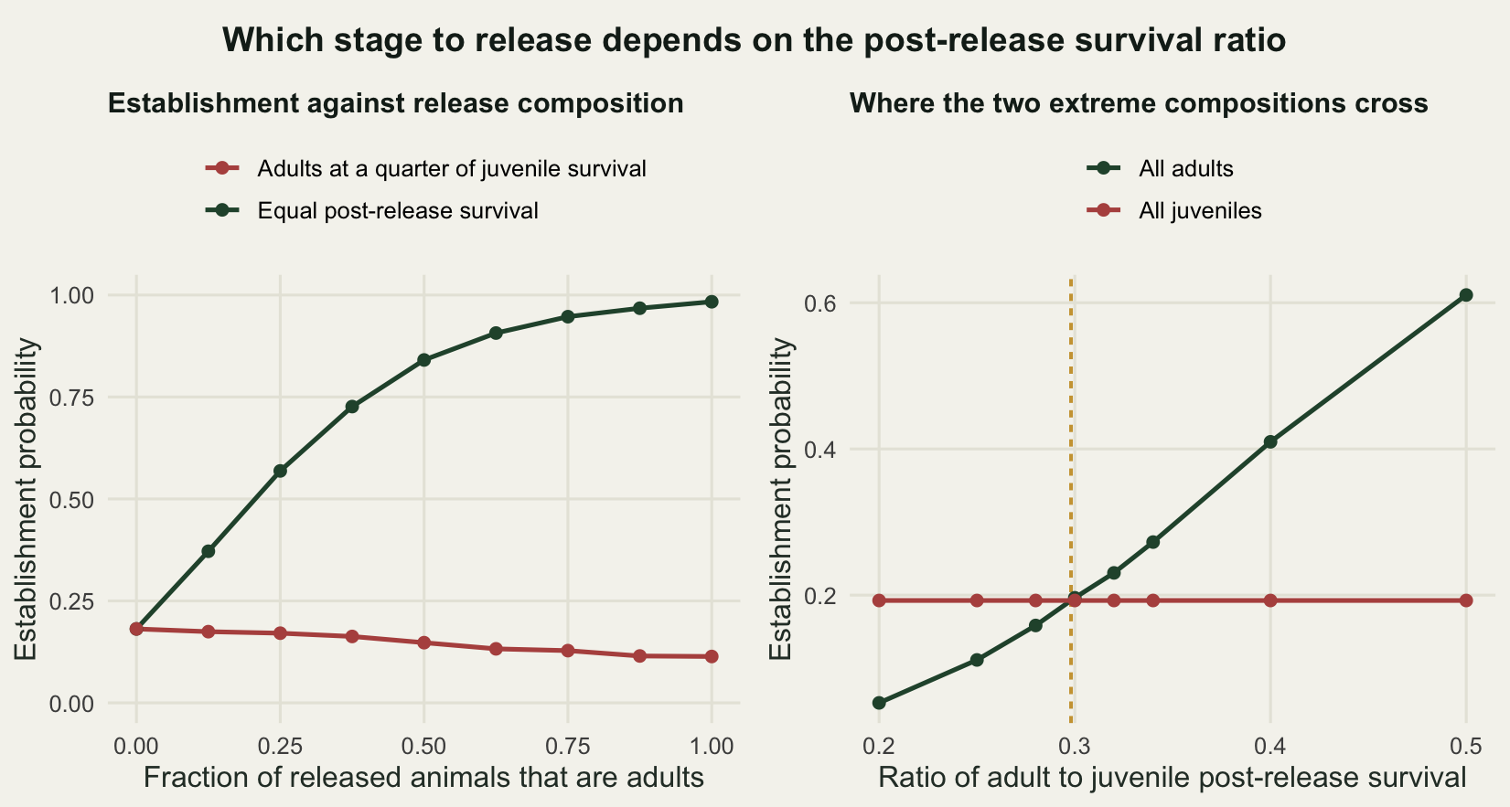
The measured crossover is at a survival ratio of 0.2981. Below it, releasing juveniles beats releasing adults; above it, adults win. The value predicted from the matrix alone, without any simulation, is the ratio of reproductive values: a juvenile is worth 0.3006 of an adult, so an adult can afford to be only about a third as likely to survive the release and still be the better animal to send. The difference between the simulated and predicted crossover is -0.0025, which is measured in units of the survival ratio, while the Monte Carlo standard error of 0.0046 is measured in units of probability, so the two do not compare directly. That standard error is a worst case as well: it is the value at one half, and the probabilities either side of the crossover sit near 0.1927, where the error is smaller. The conversion comes from the diff column, which runs from 0.0037 at a ratio of 0.30 to 0.0377 at 0.32, so an error of 0.0046 in probability moves the crossover by well under 0.01 in ratio, and on this run the gap between simulation and prediction is no bigger than that. Some of that agreement is luck at this replicate count, but the argument behind it is not: the left eigenvector prices a released animal, and a post-release survival multiplier is a discount on that price.
This is the practical result of the post. The composition decision does not need a simulation at all if the post-release survival ratio is known: compute the reproductive values, compare the ratio, and send the stage that comes out ahead. What does need measuring is the survival ratio itself, and the number of reintroduction programmes that have a defensible estimate of it is small. A ratio of 0.30 is not an extreme assumption for a territorial mammal or a long-lived bird, so a composition decision made on reproductive values alone, with equal post-release survival assumed, is being made near the point where its own answer changes sign.
The marginal animal
The last decision variable is the total. Fix the schedule at five years and the composition at half adults, with equal post-release survival, and sweep the total from 10 to 200 in steps of ten. The quantity a programme actually needs is not the curve but its slope: what does the next animal buy.
tot_grid <- seq(10, 200, by = 10)
nrep_tot <- 20000
p_tot <- sapply(tot_grid, function(x)
  run_release(x, 5, 0.5, phi_base, phi_base, nrep_tot)$p_est)
marg <- c(NA, diff(p_tot) / 10)

cut_marg <- 0.002
below <- which(!is.na(marg) & marg < cut_marg)
first_stable <- tot_grid[min(below[sapply(below, function(i)
  all(marg[i:length(marg)] < cut_marg))])]

print(c(replicates = nrep_tot, marginal_cutoff = cut_marg,
        n_totals = length(tot_grid)))
replicates marginal_cutoff n_totals
2e+04 2e-03 2e+01 print(round(data.frame(total = tot_grid, p_est = p_tot,
gain_per_animal = marg), 5)) total p_est gain_per_animal
1 10 0.00010 NA
2 20 0.00395 0.00039
3 30 0.02025 0.00163
4 40 0.06230 0.00421
5 50 0.13015 0.00678
6 60 0.23645 0.01063
7 70 0.35490 0.01184
8 80 0.47785 0.01230
9 90 0.59235 0.01145
10 100 0.69470 0.01023
11 110 0.77380 0.00791
12 120 0.83845 0.00646
13 130 0.88345 0.00450
14 140 0.92320 0.00398
15 150 0.94290 0.00197
16 160 0.96070 0.00178
17 170 0.97110 0.00104
18 180 0.98150 0.00104
19 190 0.98585 0.00043
20 200 0.99010 0.00042print(round(c(gain_at_40 = marg[tot_grid == 40],
gain_at_100 = marg[tot_grid == 100],
gain_at_180 = marg[tot_grid == 180],
diminishing_returns_total = first_stable,
p_at_that_total = p_tot[tot_grid == first_stable],
p_at_200 = p_tot[tot_grid == 200]), 5)) gain_at_40 gain_at_100 gain_at_180
0.00421 0.01023 0.00104
diminishing_returns_total p_at_that_total p_at_200
150.00000 0.94290 0.99010 The curve is sigmoid, which is why the marginal animal is worth wildly different amounts depending on where you are on it. The last ten animals of a release of 40 raise the establishment probability by 0.00421 each. The last ten of a release of 100 are worth 0.01023 each, more than twice as much. The last ten of a release of 180 are worth 0.00104 each, a fraction of their value at 40 and a smaller fraction still of their value at 100.
Take 0.002 of establishment probability per animal as the point at which an animal is no longer worth taking from the donor population. The marginal gain first falls below that value, and stays below it for every larger total, at a release of 150 animals, where the establishment probability is 0.9429. Pushing the total to 200 animals raises it to 0.9901, so the whole stretch from 150 to 200 buys less than five points of establishment probability.
That is a stopping rule, and it is a defensible one, because the animals are not free. They come out of a donor population that has its own extinction risk, or out of a captive programme whose capacity is the binding constraint on every other project it runs. A release that stops at 150 and puts the animals it did not use into a second site, or leaves them in the donor population, is making better use of them than a release that pushes a single site from 0.9429 to 0.9901. The cutoff of 0.002 is a value judgement and it should be argued rather than assumed, but the shape of the curve that makes it bite is a measurement.
What this cannot tell you
Every number above assumes the reason the species disappeared has been fixed. The deterministic growth rate is 1.0405, so the modelled habitat supports a growing population and the only question is whether the founders survive long enough to get there. Reintroductions fail for that reason less often than they fail because the original problem is still present.
Model the residual problem as reduced breeding output, enough to bring the deterministic growth rate just below one, and then run the entire optimisation again: all four schedules, five compositions, at each of five totals, and take the best result at each total. If any allocation can rescue a site that is still slightly hostile, this sweep will find it.
fec_deg <- 0.53
lam_deg <- Re(eigen(make_A(fec_deg))$values[1])
deg_tot <- c(40, 80, 120, 160, 200)
nrep_deg <- 4000

deg_best <- t(sapply(deg_tot, function(x) {
  grid_s <- expand.grid(k = sched, f = seq(0, 1, by = 0.25))
  vals <- mapply(function(k, f)
    run_release(x, k, f, phi_base, phi_base, nrep_deg, fecundity = fec_deg,
                years = 50, check = c(25, 50))$p_est,
    grid_s$k, grid_s$f)
  c(total = x, best_25 = max(vals[1, ]), worst_25 = min(vals[1, ]),
    best_50 = max(vals[2, ]))
}))

print(c(replicates = nrep_deg, degraded_fecundity = fec_deg,
        strategies_per_total = length(sched) * 5))
replicates degraded_fecundity strategies_per_total
4000.00 0.53 20.00 print(round(c(lambda_degraded = lam_deg, lambda_intact = lambda), 4))lambda_degraded lambda_intact
0.9809 1.0405 print(round(as.data.frame(deg_best), 4)) total best_25 worst_25 best_50
1 40 0.0000 0 0.0000
2 80 0.0015 0 0.0015
3 120 0.0367 0 0.0068
4 160 0.1688 0 0.0310
5 200 0.4185 0 0.0750print(round(c(healthy_120 = p_tot[tot_grid == 120],
degraded_best_120 = deg_best[deg_best[, "total"] == 120, "best_25"],
degraded_best_200_25y = deg_best[deg_best[, "total"] == 200, "best_25"],
degraded_best_200_50y = deg_best[deg_best[, "total"] == 200, "best_50"]), 4)) healthy_120 degraded_best_120.best_25
0.8384 0.0367
degraded_best_200_25y.best_25 degraded_best_200_50y.best_50
0.4185 0.0750 tot_long <- rbind(
data.frame(total = tot_grid, p = p_tot,
case = "Habitat fixed, growth rate 1.0405"),
data.frame(total = deg_best[, "total"], p = deg_best[, "best_25"],
case = "Residual problem, growth rate 0.9809 (best of 20 strategies)"))
ggplot(tot_long, aes(total, p, colour = case)) +
geom_vline(xintercept = first_stable, colour = te_pal$gold,
linewidth = 0.7, linetype = "22") +
geom_line(linewidth = 0.9) +
geom_point(size = 1.9) +
scale_colour_manual(values = c(te_pal$forest, te_pal$clay), name = NULL) +
coord_cartesian(ylim = c(0, 1)) +
labs(x = "Total animals released", y = "Establishment probability",
title = "Allocation cannot substitute for a habitat that still fails") +
theme_te() +
theme(legend.position = "top", legend.direction = "vertical")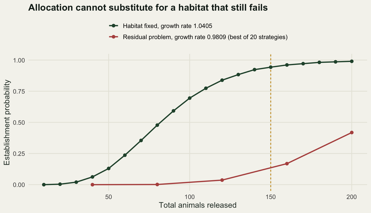
With the residual problem in place the deterministic growth rate is 0.9809, a decline of under two per cent a year, which is well inside the error bars of most field estimates of survival. The best establishment probability over all twenty allocations is 0.0000 at a total of 40, 0.0015 at 80, 0.0367 at 120, 0.1688 at 160 and 0.4185 at 200. Compare the intact case, where 120 animals gave 0.8384. At the total where a working habitat returns 0.8384, a habitat losing two per cent a year returns 0.0367, and no schedule and no stage composition changes that. The worst strategy and the best strategy at a total of 120 differ by less than the gap between either of them and the intact case.
The one number that does not behave is at the largest total. Releasing 200 animals into a declining habitat gives an establishment probability of 0.4185 at year 25, which looks like a partial success. It is not. Check the same runs at year 50 and the probability of still being above 100 individuals is 0.0750. What the 25-year figure is measuring there is inertia: 200 animals released into a population declining at under two per cent a year takes decades to fall through a threshold of 100, and the establishment criterion cannot tell the difference between a population that is growing and a large one that is going down slowly. A reintroduction can be declared established, on a criterion agreed in advance and applied honestly, and still be a population in decline with a stated endpoint.
That failure belongs to the criterion, not to the model, and it is the reason to state the threshold and the horizon at the start and then argue about them. A horizon of 25 years is short relative to the generation time of most species that get reintroduced. If the horizon cannot be lengthened, then establishment should be defined on the growth rate over the last part of the projection rather than on the population size at its end, because size at a fixed date is a quantity you can buy.
Three further limits are worth naming without pretending they were measured here. There is no density dependence in the model, so a successful population grows without a ceiling and the establishment probabilities at large totals are optimistic about the later years. There is no genetics, so the founder number appears only through demography and not through inbreeding, which argues in the same direction as spreading releases and would push the schedule optimum later. And release-year quality is the only correlated risk, so environmental variation among ordinary years is missing, which makes every establishment probability here higher than it should be.
Where to go next
The obvious next step is to test whether the machinery above survives contact with the checks that catch this kind of model out, which is what checking a reintroduction analysis does. The other direction is spatial: this post allocated animals along the axes of time and stage, and the same fixed budget can be allocated across sites instead, which is the same optimisation with a different currency and is treated in the reserve configuration post below.
References
Armstrong DP, Seddon PJ 2008 Trends in Ecology and Evolution 23(1):20-25 (10.1016/j.tree.2007.10.003)
Griffith B, Scott JM, Carpenter JW, Reed C 1989 Science 245(4917):477-480 (10.1126/science.245.4917.477)
Deredec A, Courchamp F 2007 Ecoscience 14(4):440-451 (10.2980/1195-6860(2007)14[440:IOTAEF]2.0.CO;2)
Robert A, Colas B, Guigon I, Kerbiriou C, Mihoub JB, Saint-Jalme M, Sarrazin F 2015 Animal Conservation 18(5):397-406 (10.1111/acv.12188)
Caswell H 2001 Matrix Population Models: Construction, Analysis, and Interpretation. Sinauer, ISBN 978-0-87893-096-8