Placebo tests for panel causal designs

With one treated unit or a handful of clusters, the usual standard errors are not to be trusted. Two placebo procedures give honest inference instead: permuting the treatment across space for synthetic control, and moving it back in time for difference-in-differences.

The three earlier posts in this batch estimated effects; this one asks whether those estimates could have arisen by chance. That question is awkward for panel designs with very few treated units. The synthetic control post had a single treated region, so there is no sample of treated units to form a sampling distribution. Difference-in-differences with a small number of clusters has a related problem: the model-based standard errors assume many independent groups and are far too small when there are not. In both cases the honest move is a placebo test. Re-run the whole analysis under conditions where the effect is known to be absent, and see whether the real estimate stands out against that reference set.

Placebo-in-space: permuting the treatment across units

For synthetic control, the reference set is built by pretending each donor was the treated unit. Apply the identical procedure to every donor, using the remaining donors as its pool, and record how large a post-intervention gap each produces relative to its own pre-intervention fit. If the real treated unit’s gap is unremarkable against this collection of placebo gaps, the effect is not distinguishable from noise.

The natural test statistic is the ratio of post-intervention to pre-intervention root mean squared prediction error. Dividing by the pre-period error is what makes the comparison fair: a donor that never fitted well in the pre-period has a large denominator, so a large post-period gap does not by itself make it rank highly.

library(ggplot2); library(dplyr); library(tidyr)
set.seed(173)
J <- 19; Tn <- 20; T0 <- 13; tvec <- 1:Tn        # 19 donors + 1 treated; smallest p is 1/20
F1 <- scale(cumsum(rnorm(Tn, 0.04, 0.6)))[, 1]; F2 <- sin(2 * pi * tvec / 9); trend <- (tvec - mean(tvec)) / Tn
Fmat <- cbind(F1, F2, trend)
Ld <- cbind(rnorm(J, 0.6, 0.7), rnorm(J, 0.4, 0.5), rnorm(J, 0.3, 0.9)); mud <- runif(J, 3.5, 5.5)
donors <- sapply(1:J, function(j) mud[j] + Fmat %*% Ld[j, ] + rnorm(Tn, 0, 0.18)); colnames(donors) <- paste0("D", 1:J)
wtrue <- c(0.45, 0.35, 0.20); mix <- c(2, 5, 9)
Lt <- colSums(wtrue * Ld[mix, ]); mut <- sum(wtrue * mud[mix])
treated <- as.numeric(mut + Fmat %*% Lt + rnorm(Tn, 0, 0.18)) + ifelse(tvec >= T0, 0.32 * (tvec - T0 + 1), 0)

pre <- 1:(T0 - 1); post <- T0:Tn
fit_sc <- function(y, pool) {                      # convex pre-period fit of y on pool columns
  Ppre <- pool[pre, , drop = FALSE]; m <- ncol(pool)
  obj <- function(p) { w <- c(p, 1 - sum(p)); mean((y[pre] - Ppre %*% w)^2) }
  ui <- rbind(diag(m - 1), rep(-1, m - 1)); ci <- c(rep(0, m - 1), -1)
  op <- constrOptim(rep(1 / m, m - 1), obj, grad = NULL, ui = ui, ci = ci,
                    method = "Nelder-Mead", control = list(maxit = 15000, reltol = 1e-11))
  w <- c(op$par, 1 - sum(op$par)); w[w < 1e-6] <- 0; as.numeric(pool %*% (w / sum(w)))
}
rat <- function(y, s) sqrt(mean((y[post] - s[post])^2)) / sqrt(mean((y[pre] - s[pre])^2))

synth_t <- fit_sc(treated, donors); gap_t <- treated - synth_t; ratio_t <- rat(treated, synth_t)
plac <- lapply(1:J, function(j) {                  # each donor treated in turn, pool = the others
  s <- fit_sc(donors[, j], donors[, -j, drop = FALSE])
  list(gap = donors[, j] - s, ratio = rat(donors[, j], s))
})
ratios <- c(ratio_t, sapply(plac, function(x) x$ratio))
pval <- mean(ratios >= ratio_t)                    # rank of treated among J+1 units
att_t <- mean(gap_t[post])

The treated region’s error ratio is 10.8, against a placebo median of 1.5: its post-intervention gap is more than ten times its pre-intervention error, whereas a typical placebo barely changes. It ranks first of 20 units, giving a permutation p-value of 0.050. With 19 donors the smallest attainable value is 0.050, so ranking first is as strong as this design allows: the estimated effect of 1.23 is not something the donors reproduce by chance.

te <- list(ink="#16241d",body="#2c3a31",forest="#275139",label="#46604a",sage="#93a87f",paper="#f5f4ee",
           line="#dad9ca",faint="#5d6b61",grazed="#cda23f",mown="#2f8f63",aband="#b5534e")
th <- theme_minimal(base_size = 12) + theme(text = element_text(colour = te$body),
  plot.title = element_text(colour = te$ink, face = "bold"), plot.subtitle = element_text(colour = te$faint, size = rel(0.9)),
  axis.title = element_text(colour = te$label), axis.text = element_text(colour = te$faint), panel.grid.minor = element_blank(),
  panel.grid.major = element_line(colour = te$line, linewidth = 0.3), legend.position = "bottom", legend.title = element_blank(),
  legend.text = element_text(colour = te$faint, size = rel(0.8)), strip.text = element_text(colour = te$ink, face = "bold"),
  plot.background = element_rect(fill = te$paper, colour = NA), panel.background = element_rect(fill = te$paper, colour = NA))
plac_gaps <- do.call(rbind, lapply(1:J, function(j) data.frame(t = tvec, gap = plac[[j]]$gap, who = paste0("D", j))))
tr_gap <- data.frame(t = tvec, gap = gap_t)
ggplot() +
  annotate("rect", xmin = T0 - 0.5, xmax = Tn + 0.5, ymin = -Inf, ymax = Inf, fill = te$sage, alpha = 0.12) +
  geom_hline(yintercept = 0, colour = te$faint, linewidth = 0.4) +
  geom_vline(xintercept = T0 - 0.5, colour = te$faint, linetype = "22", linewidth = 0.5) +
  geom_line(data = plac_gaps, aes(t, gap, group = who), colour = te$line, linewidth = 0.4) +
  geom_line(data = tr_gap, aes(t, gap), colour = te$aband, linewidth = 1.1) +
  geom_point(data = tr_gap, aes(t, gap), colour = te$aband, size = 1.2) +
  annotate("text", x = 1, y = max(tr_gap$gap) * 0.9, hjust = 0, colour = te$aband, size = 3.3,
           label = sprintf("treated region\nRMSPE ratio = %.1f\npermutation p = %.3f", ratio_t, pval)) +
  labs(x = "Year", y = "Gap: unit minus its synthetic control",
       title = "Placebo-in-space: the treated gap stands out from the donor placebos",
       subtitle = "Grey: each donor treated as a placebo. The treated region (red) departs only after the intervention.") + th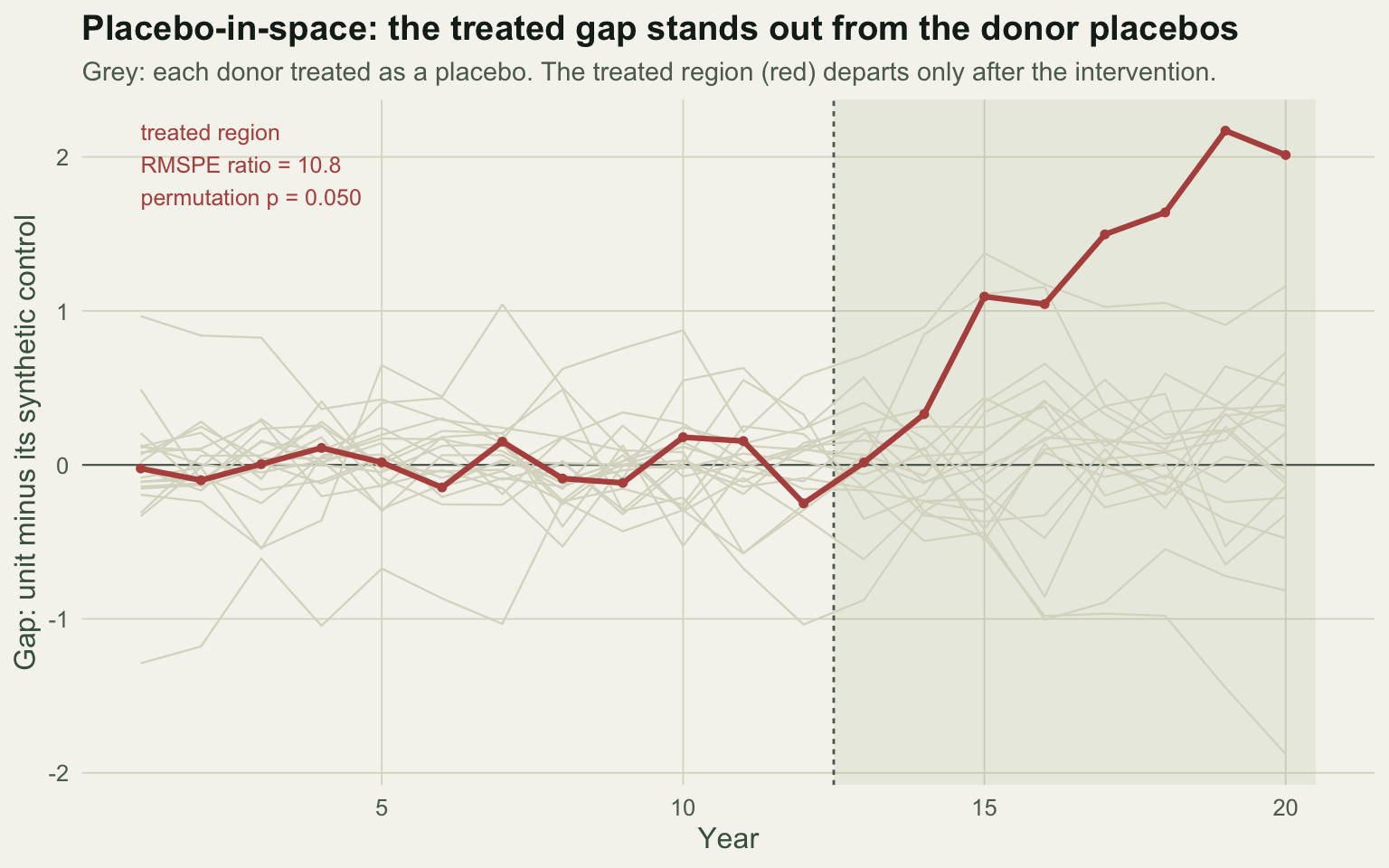

Figure 1: Each grey line is a donor’s gap when it is treated as a placebo; the bold red line is the real treated region. The treated gap sits among the placebos before the intervention and separates sharply afterwards.

Placebo-in-time: moving the treatment into the past

The second placebo keeps the treated and control groups fixed but shifts the intervention date. Restrict the data to periods before the real intervention, declare a fake adoption partway through that pre-period, and estimate the difference-in-differences. Nothing happened at the fake date, so under parallel trends the placebo estimate should be a precise zero. If it is not, the two groups were already drifting apart, and the design is in trouble regardless of what the real estimate says.

set.seed(2718)
Ndid <- 40; Ty <- 14; Tt <- 9; trt <- 1:20        # real adoption in year 9
al <- rnorm(Ndid, 0, 0.7); gt <- cumsum(c(0, rnorm(Ty - 1, 0.04, 0.12)))
mkp <- function(ptr) {
  d <- expand.grid(id = 1:Ndid, year = 1:Ty); d$treated <- as.integer(d$id %in% trt)
  eff <- ifelse(d$treated == 1 & d$year >= Tt, 0.9, 0)
  tr <- ifelse(d$treated == 1, ptr * (d$year - Tt), 0)
  d$y <- al[d$id] + gt[d$year] + eff + tr + rnorm(nrow(d), 0, 0.35); d
}
did_est <- function(d) {
  co <- summary(lm(y ~ factor(id) + factor(year) + post:treated, d))$coefficients["post:treated", ]
  c(b = unname(co[1]), se = unname(co[2]), p = unname(co[4]))
}
Tp <- 5                                            # fake adoption in year 5
real_time <- function(d) { d$post <- as.integer(d$year >= Tt); did_est(d) }
placebo_time <- function(d) { dd <- subset(d, year < Tt); dd$post <- as.integer(dd$year >= Tp); did_est(dd) }

Run this on two datasets: one with parallel trends, one with a small differential trend of 0.15 index units per year in the treated group.

d_clean <- mkp(0); d_ptr <- mkp(0.15)
rc <- real_time(d_clean); pc <- placebo_time(d_clean)
rp <- real_time(d_ptr);   pp <- placebo_time(d_ptr)

Under parallel trends the real estimate is 1.00 (p < 0.001) and the placebo is 0.01 (p = 0.88): a clean null exactly where there should be one. Under the pre-trend the real estimate inflates to 1.87, but now the placebo is 0.54 and significant (p < 0.001). The placebo has caught the drift using pre-intervention data alone, before the real estimate could be mistaken for an effect.

d2 <- data.frame(
  scenario = rep(c("Parallel trends hold", "Differential pre-trend"), each = 2),
  which = rep(c("real (year 9)", "placebo (year 5)"), 2),
  b = c(rc["b"], pc["b"], rp["b"], pp["b"]), se = c(rc["se"], pc["se"], rp["se"], pp["se"]),
  p = c(rc["p"], pc["p"], rp["p"], pp["p"]))
d2$scenario <- factor(d2$scenario, levels = c("Parallel trends hold", "Differential pre-trend"))
d2$which <- factor(d2$which, levels = c("placebo (year 5)", "real (year 9)"))
d2$lo <- d2$b - 1.96 * d2$se; d2$hi <- d2$b + 1.96 * d2$se
d2$lab <- ifelse(d2$p < 0.001, "p<0.001", sprintf("p=%.3f", d2$p))
ggplot(d2, aes(b, which, colour = which)) +
  geom_vline(xintercept = 0, colour = te$faint, linewidth = 0.4) +
  geom_errorbarh(aes(xmin = lo, xmax = hi), height = 0.16, linewidth = 0.5) +
  geom_point(size = 2.8) + geom_text(aes(label = lab), vjust = -1.1, size = 3, show.legend = FALSE) +
  facet_wrap(~scenario, ncol = 1) +
  scale_colour_manual(values = c("real (year 9)" = te$mown, "placebo (year 5)" = te$grazed)) +
  labs(x = "Difference-in-differences estimate", y = NULL,
       title = "Placebo-in-time: a fake pre-period adoption should show no effect",
       subtitle = "Under parallel trends the placebo is null; under a pre-trend the placebo is significant, exposing the design.") +
  th + theme(legend.position = "none")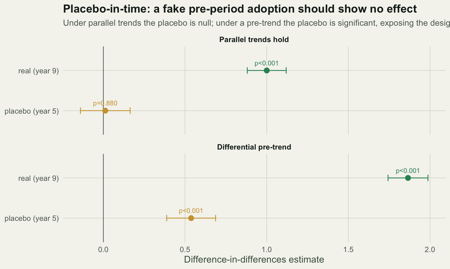

Warning: `geom_errorbarh()` was deprecated in ggplot2 4.0.0.
ℹ Please use the `orientation` argument of `geom_errorbar()` instead.

`height` was translated to `width`.

Figure 2: Real and placebo difference-in-differences estimates under each scenario. The placebo is a precise zero when trends are parallel and clearly non-zero when they are not, flagging the design as unreliable.

The limits of a placebo

Placebo inference is honest but blunt, and it should be read with three cautions. Its validity rests on exchangeability: the permutation logic assumes that under the null the treated unit is not systematically different from the donors, which fails if the treated region was selected precisely because it was unusual. The p-value is coarse when units are few, bounded below by one over the number of units, so a single treated region against nineteen donors cannot report anything smaller than 0.05 no matter how clean the separation. And a placebo can only refute, not confirm: a null placebo-in-time is consistent with parallel trends but does not prove it, exactly as the pre-trend test in the event-study post could screen for violations without guaranteeing their absence.

None of this makes the tests optional. For a single treated unit there is often no credible alternative to a permutation, and a placebo that moves the treatment in time is among the cheapest checks available for any difference-in-differences. Reporting them, and reporting them when they fail, is what separates a comparative case study that has been stress-tested from one that merely looks convincing.

Related tutorials

• The synthetic control method
• Event-study difference-in-differences
• Staggered adoption and two-way fixed-effects bias
• Before-after-control-impact and difference-in-differences

References

• Abadie, A., Diamond, A. and Hainmueller, J. (2010). Synthetic control methods for comparative case studies: estimating the effect of California’s tobacco control program. Journal of the American Statistical Association, 105(490), 493-505. https://doi.org/10.1198/jasa.2009.ap08746
• Abadie, A. (2021). Using synthetic controls: feasibility, data requirements, and methodological aspects. Journal of Economic Literature, 59(2), 391-425. https://doi.org/10.1257/jel.20191450
• Bertrand, M., Duflo, E. and Mullainathan, S. (2004). How much should we trust differences-in-differences estimates? Quarterly Journal of Economics, 119(1), 249-275. https://doi.org/10.1162/003355304772839588
• Conley, T.G. and Taber, C.R. (2011). Inference with difference in differences with a small number of policy changes. Review of Economics and Statistics, 93(1), 113-125. https://doi.org/10.1162/REST_a_00049
• Ferman, B. and Pinto, C. (2019). Inference in differences-in-differences with few treated groups and heteroskedasticity. Review of Economics and Statistics, 101(3), 452-467. https://doi.org/10.1162/rest_a_00759
• Larsen, A.E., Meng, K. and Kendall, B.E. (2019). Causal analysis in control-impact ecological studies with observational data. Methods in Ecology and Evolution, 10(7), 924-934. https://doi.org/10.1111/2041-210X.13190

References

- Abadie A, Diamond A, Hainmueller J 2010 Journal of the American Statistical Association 105(490):493-505 (10.1198/jasa.2009.ap08746)
- Abadie A 2021 Journal of Economic Literature 59(2):391-425 (10.1257/jel.20191450)
- Bertrand M, Duflo E, Mullainathan S 2004 Quarterly Journal of Economics 119(1):249-275 (10.1162/003355304772839588)
- Conley TG, Taber CR 2011 Review of Economics and Statistics 93(1):113-125 (10.1162/REST_a_00049)
- Ferman B, Pinto C 2019 Review of Economics and Statistics 101(3):452-467 (10.1162/rest_a_00759)
- Larsen AE, Meng K, Kendall BE 2019 Methods in Ecology and Evolution 10(7):924-934 (10.1111/2041-210X.13190)