library(ggplot2); library(dplyr); library(tidyr)
set.seed(88)
Tn <- 12; npg <- 20; tg <- c(4, 7, 10); N <- 4 * npg
idL <- list(); for (i in seq_along(tg)) idL[[i]] <- ((i - 1) * npg + 1):(i * npg)
gvec <- rep(NA_integer_, N); for (i in seq_along(tg)) gvec[idL[[i]]] <- tg[i]   # NA = never-treated
att_dyn <- function(e) ifelse(e < 0, 0, 0.25 * (e + 1))                          # true dynamic effect
alph <- rnorm(N, 0, 0.7); lam <- cumsum(c(0, rnorm(Tn - 1, 0.03, 0.10))); sig <- 0.30
d <- expand.grid(id = 1:N, year = 1:Tn)
d$g <- gvec[d$id]; d$e <- ifelse(is.finite(d$g), d$year - d$g, NA_integer_)
d$D <- as.integer(is.finite(d$g) & d$year >= d$g)                                # treated-now
d$eff <- ifelse(d$D == 1, att_dyn(d$e), 0)
d$y <- alph[d$id] + lam[d$year] + d$eff + rnorm(nrow(d), 0, sig)
true_att <- mean(d$eff[d$D == 1]) # true overall ATTStaggered adoption and two-way fixed effects
causal inference
ecology tutorial
R
When units are treated at different times, two-way fixed effects quietly uses already-treated units as controls, and those forbidden comparisons go negative.
The event-study post treated a single adoption date. Programmes rarely roll out that way. Reserves join a restoration scheme in different years; sites adopt a management change on their own schedule. The natural reflex is to keep the same regression, unit fixed effects plus year fixed effects plus one treatment indicator, and read off the coefficient. With staggered timing and an effect that changes over time, that coefficient is not the average treatment effect. It can be badly wrong, and the reason is subtle enough that it went unnoticed in applied work for years.
A staggered restoration rollout
Take 80 sites over 12 years. Three cohorts of 20 adopt a restoration treatment in years 4, 7 and 10; the remaining 20 never adopt. The treatment effect builds up the same way in every cohort: 0.25 index units in the adoption year, rising by another 0.25 for every year that follows. Site levels and a shared year trend are common across groups.
The overall average treatment effect on the treated, averaged over every treated site-year, is 1.00. Now fit the ordinary two-way fixed-effects model.
m_twfe <- lm(y ~ factor(id) + factor(year) + D, d)
b_twfe <- coef(m_twfe)["D"]; se_twfe <- summary(m_twfe)$coefficients["D", "Std. Error"]
It returns 0.47 (standard error 0.049), less than half the true effect of 1.00. The estimate is precise and badly biased at the same time, so nothing in its own output warns you.
Why: the forbidden comparisons
Goodman-Bacon (2021) showed that the two-way fixed-effects coefficient is a weighted average of all the two-by-two difference-in-differences you can form between timing groups. Some of those are clean: a cohort compared with the never-treated, or an earlier cohort compared with a later one while the later one is still untreated. One kind is not. When a later cohort is compared against an earlier one that has already adopted, the earlier group is not a valid control, because its outcome is still moving as its own treatment effect grows. Under a dynamic effect that changing control contaminates the comparison, and the two-by-two can even come out negative.
gm <- function(I, Y) mean(d$y[d$id %in% I & d$year %in% Y])
io <- function(g) which(gvec == g); inev <- which(!is.finite(gvec))
bacon <- list()
for (g in tg) {                                     # treated vs never (clean)
  post <- g:Tn; pre <- 1:(g - 1)
  did <- (gm(io(g), post) - gm(io(g), pre)) - (gm(inev, post) - gm(inev, pre))
  nk <- length(io(g)); nu <- length(inev); ntot <- nk + nu; sk <- nk / ntot
  w <- (sk * (1 - sk)) * (length(post) / Tn) * (length(pre) / Tn) * ntot^2
  bacon[[length(bacon) + 1]] <- data.frame(type = "treated vs never", pair = sprintf("%d", g), did = did, w = w, forbidden = FALSE)
}
for (a in 1:(length(tg) - 1)) for (b in (a + 1):length(tg)) {
  k <- tg[a]; l <- tg[b]
  win <- k:(l - 1); pre <- 1:(k - 1)                # early treated vs later not-yet (clean)
  did1 <- (gm(io(k), win) - gm(io(k), pre)) - (gm(io(l), win) - gm(io(l), pre))
  nk <- length(io(k)); nl <- length(io(l)); ntot <- nk + nl; sk <- nk / ntot
  w1 <- (sk * (1 - sk)) * (length(win) / Tn) * (length(pre) / Tn) * ntot^2
  bacon[[length(bacon) + 1]] <- data.frame(type = "early vs later-control", pair = sprintf("%d|%d", k, l), did = did1, w = w1, forbidden = FALSE)
  win2 <- l:Tn; pre2 <- k:(l - 1)                   # late treated vs already-treated early (forbidden)
  did2 <- (gm(io(l), win2) - gm(io(l), pre2)) - (gm(io(k), win2) - gm(io(k), pre2))
  w2 <- (sk * (1 - sk)) * (length(win2) / Tn) * (length(pre2) / Tn) * ntot^2
  bacon[[length(bacon) + 1]] <- data.frame(type = "late vs already-treated", pair = sprintf("%d|%d", l, k), did = did2, w = w2, forbidden = TRUE)
}
B <- do.call(rbind, bacon); B$w <- B$w / sum(B$w)
twfe_recon <- sum(B$w * B$did)
wforb <- sum(B$w[B$forbidden]); maxforb <- max(B$did[B$forbidden]); minforb <- min(B$did[B$forbidden])
The weighted average of these two-by-two estimates reproduces the regression coefficient exactly: 0.467 against 0.467. That identity is the whole point. The clean comparisons are all positive, but the three forbidden “late versus already-treated” comparisons are all negative (from -0.64 to -0.27), and they carry 25% of the total weight. Every Goodman-Bacon weight is positive, here and in general; what turns negative is the comparison itself, and that block is what drags the coefficient down to 0.47.
te <- list(ink="#16241d",body="#2c3a31",forest="#275139",label="#46604a",sage="#93a87f",paper="#f5f4ee",
           line="#dad9ca",faint="#5d6b61",grazed="#cda23f",mown="#2f8f63",aband="#b5534e")
th <- theme_minimal(base_size = 12) + theme(text = element_text(colour = te$body),
  plot.title = element_text(colour = te$ink, face = "bold"), plot.subtitle = element_text(colour = te$faint, size = rel(0.9)),
  axis.title = element_text(colour = te$label), axis.text = element_text(colour = te$faint), panel.grid.minor = element_blank(),
  panel.grid.major = element_line(colour = te$line, linewidth = 0.3), legend.position = "bottom",
  legend.text = element_text(colour = te$faint, size = rel(0.8)),
  plot.background = element_rect(fill = te$paper, colour = NA), panel.background = element_rect(fill = te$paper, colour = NA))
ggplot(B, aes(w, did, colour = type, size = w)) +
  geom_hline(yintercept = 0, colour = te$faint, linewidth = 0.4) +
  geom_hline(aes(yintercept = b_twfe, linetype = "TWFE weighted average"), colour = te$grazed, linewidth = 0.8) +
  geom_hline(aes(yintercept = true_att, linetype = "True overall ATT"), colour = te$forest, linewidth = 0.8) +
  geom_point(alpha = 0.9) + geom_text(aes(label = pair), size = 2.7, vjust = -1.1, show.legend = FALSE) +
  scale_colour_manual(values = c("treated vs never" = te$mown, "early vs later-control" = te$sage, "late vs already-treated" = te$aband), name = NULL) +
  scale_linetype_manual(values = c("TWFE weighted average" = "solid", "True overall ATT" = "31"), name = NULL) +
  scale_size(range = c(2.5, 6), guide = "none") + guides(colour = guide_legend(nrow = 2, override.aes = list(size = 3))) +
  labs(x = "Goodman-Bacon weight", y = "2x2 difference-in-differences estimate",
       title = "TWFE is a weighted average of 2x2 comparisons",
       subtitle = "The red 'late vs already-treated' comparisons turn negative under a growing effect\nand drag TWFE below the truth.") + th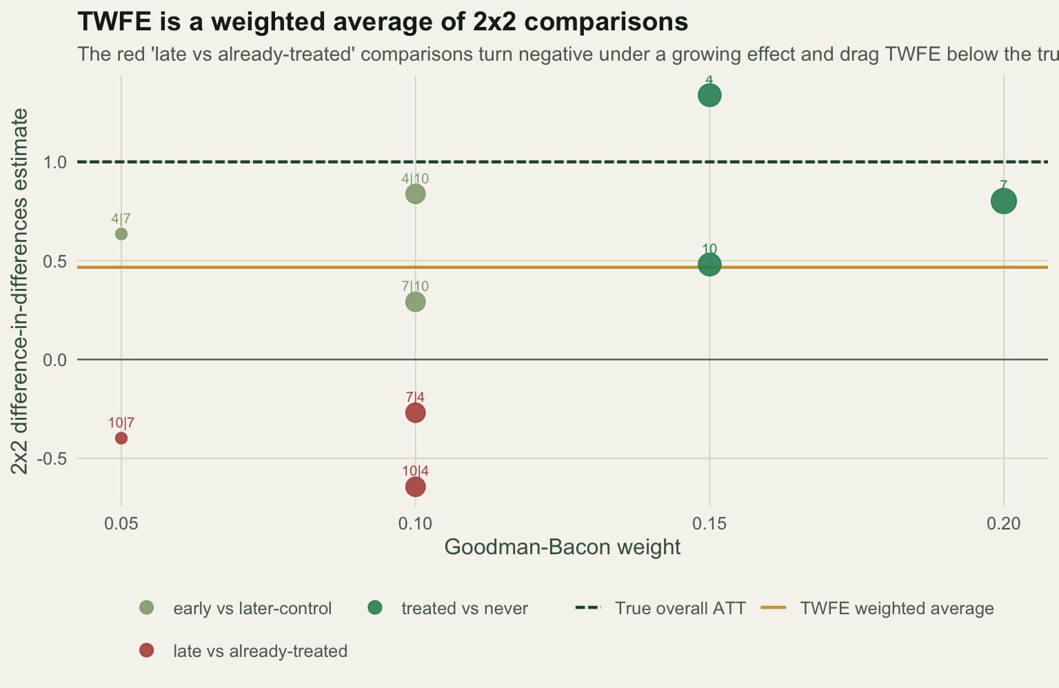
The fix: group-time effects with clean controls
The repair is to stop pooling and estimate the effect for each cohort at each period separately, using only units that are not yet treated as controls. This is the Callaway and Sant’Anna (2021) group-time average treatment effect. For cohort g observed at time t, take the change in the cohort’s outcome from the period before adoption to t, and subtract the same change for units still untreated at t. No already-treated unit ever enters as a control, so the forbidden comparisons never happen. The group-time effects can then be averaged by event time into a dynamic path, or into a single overall number.
cs <- list()
for (g in tg) {
  base <- g - 1
  for (t in g:Tn) {
    ctrl <- setdiff(which(!is.finite(gvec) | gvec > t), io(g))    # not-yet-treated (incl never)
    cs[[length(cs) + 1]] <- data.frame(g = g, t = t, e = t - g,
      att = (gm(io(g), t) - gm(io(g), base)) - (gm(ctrl, t) - gm(ctrl, base)))
  }
}
CS <- do.call(rbind, cs)
ag <- CS %>% group_by(e) %>% summarise(att = mean(att), .groups = "drop"); ag$true <- att_dyn(ag$e)
cs_overall <- mean(CS$att); maxdev <- max(abs(ag$att - ag$true))
Averaged by event time, the group-time estimator tracks the true growing effect at every horizon (largest deviation 0.09), and the overall average comes out at 1.02, close to the true 1.00. The same data that gave the two-way regression 0.47 gives the heterogeneity-consistent estimator 1.02, because it refuses the comparisons that were never valid.
ggplot(ag, aes(e, att)) +
  geom_hline(yintercept = 0, colour = te$faint, linewidth = 0.4) +
  geom_hline(aes(yintercept = b_twfe, linetype = "naive TWFE"), colour = te$grazed, linewidth = 0.8) +
  geom_line(aes(y = true, colour = "true ATT(e)"), linewidth = 0.7, linetype = "31") +
  geom_point(aes(y = true, colour = "true ATT(e)"), size = 1.4) +
  geom_line(aes(colour = "Callaway-Sant'Anna"), linewidth = 0.7) +
  geom_point(aes(colour = "Callaway-Sant'Anna"), size = 2.4) +
  annotate("text", x = 6.2, y = b_twfe - 0.14, label = sprintf("naive TWFE = %.2f", b_twfe), colour = te$grazed, size = 3.1) +
  scale_colour_manual(values = c("Callaway-Sant'Anna" = te$mown, "true ATT(e)" = te$forest), name = NULL) +
  scale_linetype_manual(values = c("naive TWFE" = "solid"), name = NULL) + scale_x_continuous(breaks = 0:8) +
  labs(x = "Event time (years since adoption)", y = "Average treatment effect on the treated",
       title = "A heterogeneity-consistent estimator recovers the dynamic effect",
       subtitle = "Group-time ATT with not-yet-treated controls tracks the true path; the single TWFE number does not.") + th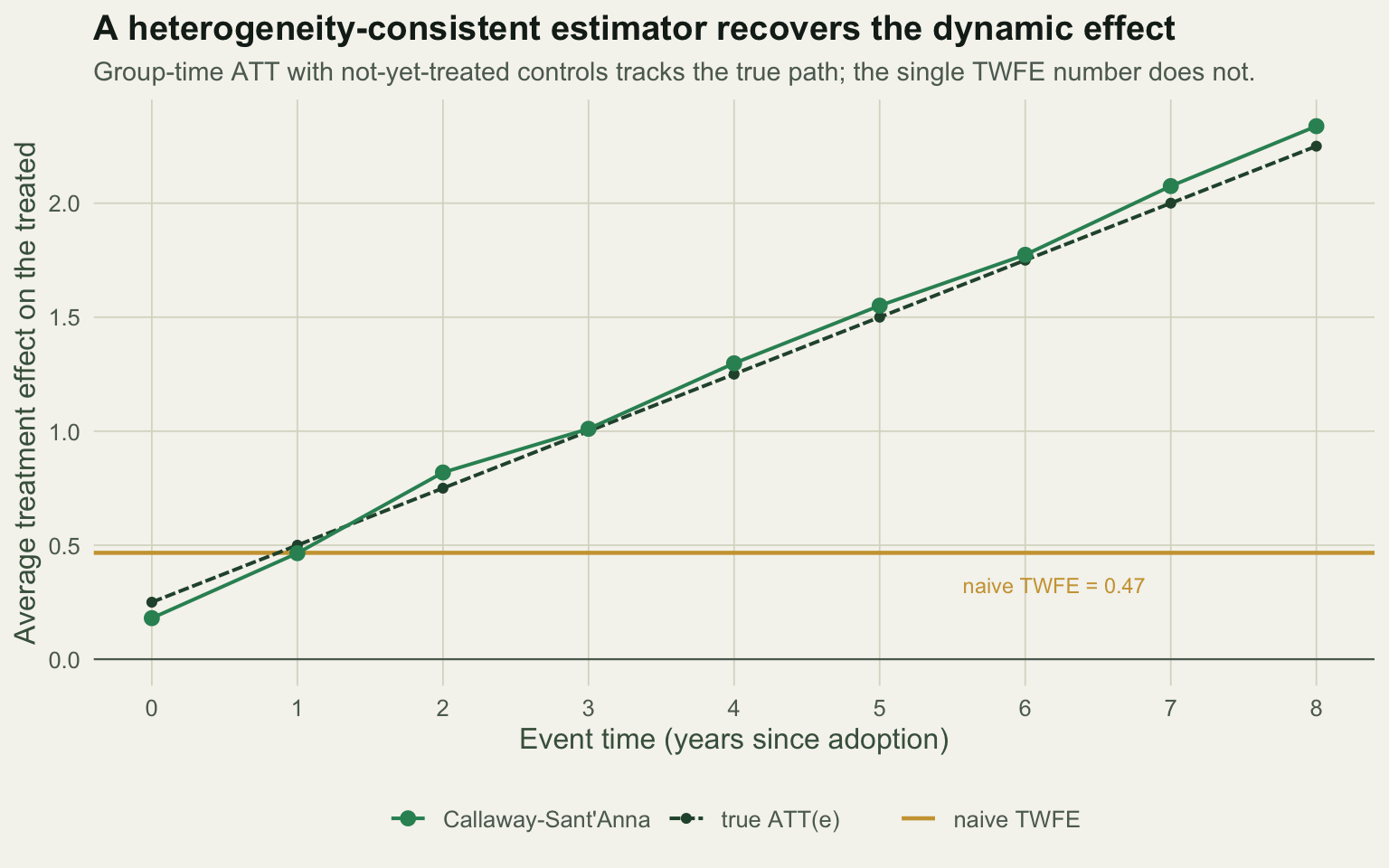
What this does and does not buy
The bias here is not a small-sample artefact and it does not average out with more data; it is built into what the two-way regression estimates when timing is staggered and effects are dynamic. The group-time approach removes it, but it leans on the same assumptions the whole design needs, and adds one of its own. It needs a clean comparison group at each period, either never-treated units or cohorts that adopt later; if almost everyone is treated early, there is little clean variation left and the estimates become fragile. It still needs parallel trends and no anticipation, now for each cohort. And it produces many group-time numbers that must be aggregated deliberately: an event-time average, a calendar-time average and a single overall effect answer different questions and can differ when effects are heterogeneous.
The last post in this series turns to inference. With one treated unit, or a handful of clusters, the usual standard errors are not trustworthy, and the honest tool is a placebo comparison rather than a formula. That also underpins the synthetic control method in the next post, which builds a tailored control for a single treated unit.
References
- Goodman-Bacon A 2021 Journal of Econometrics 225(2):254-277 (10.1016/j.jeconom.2021.03.014)
- Callaway B, Sant’Anna PHC 2021 Journal of Econometrics 225(2):200-230 (10.1016/j.jeconom.2020.12.001)
- de Chaisemartin C, D’Haultfoeuille X 2020 American Economic Review 110(9):2964-2996 (10.1257/aer.20181169)
- Sun L, Abraham S 2021 Journal of Econometrics 225(2):175-199 (10.1016/j.jeconom.2020.09.006)
- Roth J, Sant’Anna PHC, Bilinski A, Poe J 2023 Journal of Econometrics 235(2):2218-2244 (10.1016/j.jeconom.2023.03.008)
- Larsen AE, Meng K, Kendall BE 2019 Methods in Ecology and Evolution 10(7):924-934 (10.1111/2041-210X.13190)