library(ggplot2); library(dplyr); library(tidyr)
set.seed(404)
N <- 40; Tn <- 12; T0 <- 7; treated_ids <- 1:20
Kset <- setdiff((1 - T0):(Tn - T0), -1)            # event times, reference k = -1
tau_true <- c(`0` = 0.30, `1` = 0.60, `2` = 0.90, `3` = 1.10, `4` = 1.20, `5` = 1.30)
alph <- rnorm(N, 0, 0.8)                            # site fixed effects
gam  <- cumsum(c(0, rnorm(Tn - 1, 0.05, 0.15)))    # common year trend (parallel)
sig  <- 0.40

make_panel <- function(pretrend = 0) {
  d <- expand.grid(id = 1:N, year = 1:Tn)
  d$treated <- as.integer(d$id %in% treated_ids)
  eff <- ifelse(d$treated == 1 & d$year >= T0, tau_true[as.character(pmin(d$year - T0, 5))], 0)
  eff[is.na(eff)] <- 0
  ptr <- ifelse(d$treated == 1, pretrend * (d$year - T0), 0)   # optional differential trend
  d$y <- alph[d$id] + gam[d$year] + eff + ptr + rnorm(nrow(d), 0, sig)
  d
}
dc <- make_panel(0)Event-study difference-in-differences
causal inference
ecology tutorial
R
A static BACI contrast gives one number. An event study splits it into a path over time, and turns the pre-intervention periods into a parallel-trends check.
A before-after-control-impact design (see the BACI post) compares one before period with one after period across a treated and a control group. That two-by-two contrast collapses the whole response into a single average. Two things get lost. If the effect builds up or fades, the single number hides the shape. And the central assumption, that treated and control sites would have moved in parallel without the intervention, is left untested.
An event-study specification recovers both. Instead of one post dummy, it estimates a separate coefficient for each period relative to the intervention. The post-intervention coefficients trace the effect over time; the pre-intervention coefficients, which should sit on zero if trends were parallel, become a visible diagnostic.
A staggered response to a management change
Consider 40 grassland sites followed for 12 years, with a management change (livestock exclusion) applied to 20 of them in year 7. The response variable is a plant diversity index. The community reacts gradually, so the true effect grows from a small early value to a larger plateau. Site levels and a shared year trend are common to both groups, so parallel trends hold by construction here.
The estimator adds site fixed effects, year fixed effects, and one indicator per event time for the treated group, leaving out the period just before the change (k = -1) as the reference. The control sites carry zeros on every event-time indicator, so the year effects identify the common trend.
event_study <- function(d) {
  X <- sapply(Kset, function(k) as.integer(d$treated == 1 & (d$year - T0) == k))
  colnames(X) <- paste0("k", ifelse(Kset < 0, paste0("m", abs(Kset)), Kset))
  df <- cbind(d, as.data.frame(X)); lag <- colnames(X)[Kset >= 0]
  m  <- lm(as.formula(paste("y ~ factor(id) + factor(year) +", paste(colnames(X), collapse = " + "))), df)
  m0 <- lm(as.formula(paste("y ~ factor(id) + factor(year) +", paste(lag, collapse = " + "))), df)
  pt <- anova(m0, m); co <- summary(m)$coefficients
  est <- data.frame(k = Kset, b = co[colnames(X), 1], se = co[colnames(X), 2])
  est$lo <- est$b - 1.96 * est$se; est$hi <- est$b + 1.96 * est$se
  list(est = est, F = pt$F[2], p = pt$`Pr(>F)`[2], df1 = pt$Df[2], df2 = pt$Res.Df[2])
}
static_did <- function(d) {
  d$post <- as.integer(d$year >= T0)
  co <- summary(lm(y ~ factor(id) + factor(year) + post:treated, d))$coefficients["post:treated", ]
  c(b = unname(co[1]), se = unname(co[2]), lo = unname(co[1] - 1.96 * co[2]), hi = unname(co[1] + 1.96 * co[2]))
}
ec <- event_study(dc); sc <- static_did(dc); avg <- mean(tau_true)
postc <- ec$est[ec$est$k >= 0, ]; postc$true <- tau_true[as.character(postc$k)]
cover <- mean(with(postc, true >= lo & true <= hi))
The static two-by-two estimator returns a single coefficient of 0.85 (95% CI 0.70 to 1.00), close to the true average post-intervention effect of 0.90. That number is correct as an average, but it says nothing about the trajectory. The event-study coefficients recover the growing path: 0.26 in the adoption year rising to 1.28 five years on (100% interval coverage of the true path). The largest pre-intervention lead magnitude is 0.19, and a joint test that the leads are all zero gives F = 0.82, p = 0.53.
te <- list(ink="#16241d",body="#2c3a31",forest="#275139",label="#46604a",sage="#93a87f",
           paper="#f5f4ee",line="#dad9ca",faint="#5d6b61",grazed="#cda23f",mown="#2f8f63",aband="#b5534e")
ec$est$grp <- ifelse(ec$est$k < 0, "pre", "post")
truthdf <- data.frame(k = as.integer(names(tau_true)), true = as.numeric(tau_true))
ggplot(ec$est, aes(k, b)) +
  annotate("rect", xmin = -0.5, xmax = 5.5, ymin = -Inf, ymax = Inf, fill = te$sage, alpha = 0.12) +
  geom_hline(yintercept = 0, colour = te$faint, linewidth = 0.4) +
  geom_vline(xintercept = -0.5, colour = te$aband, linetype = "22", linewidth = 0.5) +
  geom_segment(data = data.frame(x = -0.5, xe = 5.5, y = sc[1]), aes(x = x, xend = xe, y = y, yend = y),
               inherit.aes = FALSE, colour = te$grazed, linewidth = 0.9) +
  annotate("text", x = -3.5, y = sc[1] + 0.12, label = sprintf("static DiD = %.2f (one average)", sc[1]),
           colour = te$grazed, size = 3.1, hjust = 0.5) +
  geom_line(data = truthdf, aes(k, true), inherit.aes = FALSE, colour = te$forest, linewidth = 0.7, linetype = "31") +
  geom_point(data = truthdf, aes(k, true), inherit.aes = FALSE, colour = te$forest, size = 1.4) +
  geom_errorbar(aes(ymin = lo, ymax = hi), width = 0.18, colour = te$ink, linewidth = 0.4) +
  geom_point(aes(fill = grp), shape = 21, colour = te$ink, size = 2.4) +
  scale_fill_manual(values = c(pre = te$paper, post = te$mown), guide = "none") +
  scale_x_continuous(breaks = Kset) +
  labs(x = "Event time (years since intervention)", y = "Effect on the index",
       title = "Event-study reveals the dynamic effect the static DiD hides",
       subtitle = "Dashed green: true path. Grey band: post-intervention. Amber line: single static-DiD coefficient.") +
  theme_minimal(base_size = 12) +
  theme(text = element_text(colour = te$body), plot.title = element_text(colour = te$ink, face = "bold"),
        plot.subtitle = element_text(colour = te$faint, size = rel(0.9)), axis.title = element_text(colour = te$label),
        axis.text = element_text(colour = te$faint), panel.grid.minor = element_blank(),
        panel.grid.major = element_line(colour = te$line, linewidth = 0.3),
        plot.background = element_rect(fill = te$paper, colour = NA), panel.background = element_rect(fill = te$paper, colour = NA))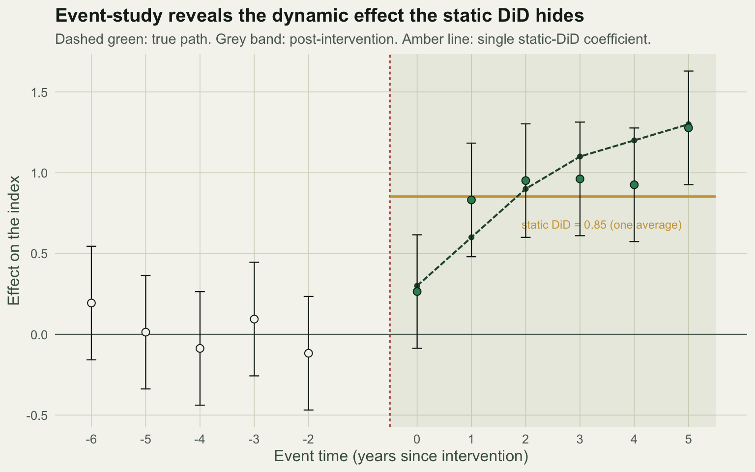
The leads are the parallel-trends check
Parallel trends cannot be verified after the intervention, because the counterfactual is never observed. What can be inspected is the period before it. If the two groups were already drifting apart, the pre-intervention leads pick up that drift and depart from zero in a systematic, trending way. Flat leads are the evidence people actually have for the assumption.
To see the failure mode, add a small differential trend to the treated group of 0.1 index units per year, present before and after the change, with the true intervention effect left unchanged.
dv <- make_panel(0.10)
ev <- event_study(dv); sv <- static_did(dv)
Now the static estimator reports 1.43 (95% CI 1.27 to 1.59), well above the true average of 0.90: the drift is absorbed into the “effect”. The event-study is where such a drift can show itself: the leads are estimated rather than assumed. Here the largest lead magnitude is 0.68, and the joint test that they are all zero gives F = 4.29, p = 0.0008.
cc <- c("k","b","se","lo","hi")
prc <- ec$est[ec$est$k < 0, cc]; prc$scenario <- "Parallel trends hold"
prv <- ev$est[ev$est$k < 0, cc]; prv$scenario <- "Differential pre-trend"
prb <- rbind(prc, prv)
prb$scenario <- factor(prb$scenario, levels = c("Parallel trends hold", "Differential pre-trend"))
labs2 <- data.frame(scenario = factor(c("Parallel trends hold", "Differential pre-trend"), levels = levels(prb$scenario)),
                    lab = c(sprintf("pre-test p = %.2f", ec$p), sprintf("pre-test p = %.3f", ev$p)), k = -6, b = 1.05)
ggplot(prb, aes(k, b)) +
  geom_hline(yintercept = 0, colour = te$faint, linewidth = 0.4) +
  geom_smooth(method = "lm", se = FALSE, colour = te$aband, linewidth = 0.5, linetype = "22", formula = y ~ x) +
  geom_errorbar(aes(ymin = lo, ymax = hi), width = 0.16, colour = te$ink, linewidth = 0.4) +
  geom_point(colour = te$ink, fill = te$sage, shape = 21, size = 2.3) +
  geom_text(data = labs2, aes(k, b, label = lab), hjust = 0, colour = te$label, size = 3.2) +
  facet_wrap(~scenario) + scale_x_continuous(breaks = (1 - T0):-2) +
  labs(x = "Event time before intervention", y = "Lead coefficient",
       title = "The pre-intervention leads are the parallel-trends check",
       subtitle = "Flat leads on zero are consistent with parallel trends; trending leads flag a violation.") +
  theme_minimal(base_size = 12) +
  theme(text = element_text(colour = te$body), plot.title = element_text(colour = te$ink, face = "bold"),
        plot.subtitle = element_text(colour = te$faint, size = rel(0.9)), axis.title = element_text(colour = te$label),
        axis.text = element_text(colour = te$faint), panel.grid.minor = element_blank(),
        panel.grid.major = element_line(colour = te$line, linewidth = 0.3), strip.text = element_text(colour = te$ink, face = "bold"),
        plot.background = element_rect(fill = te$paper, colour = NA), panel.background = element_rect(fill = te$paper, colour = NA))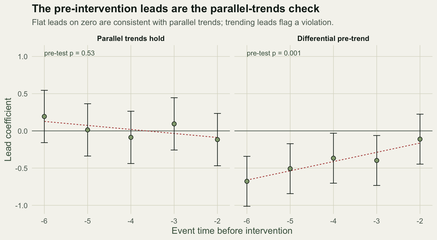
What the check can and cannot do
The pre-test is a screen, not a proof. It has two honest limits. A flat set of leads is consistent with parallel trends but does not establish them: the test is often underpowered, so a true but modest pre-trend can pass, and failing to reject is not the same as confirming the assumption. And the leads only speak to the pre-period; nothing rules out a trend that begins exactly at the intervention for reasons unrelated to it. A sensible workflow reports the full event-study path, shows the leads rather than a single number, and treats a clean pre-test as necessary but not sufficient. Where the pre-trend is worrying, a sensitivity analysis that asks how large a violation would need to be to overturn the result is the honest next step.
The event-study also sets up the harder problem in the next post. Here every treated site adopts in the same year. When adoption is staggered across cohorts, the ordinary two-way fixed-effects regression starts making comparisons it should not, and the single coefficient can mislead even when each cohort’s effect is estimated well.
References
- Angrist JD, Pischke J-S 2009 Mostly Harmless Econometrics: An Empiricist’s Companion. Princeton University Press. ISBN 978-0-691-12035-5
- Callaway B, Sant’Anna PHC 2021 Journal of Econometrics 225(2):200-230 (10.1016/j.jeconom.2020.12.001)
- Sun L, Abraham S 2021 Journal of Econometrics 225(2):175-199 (10.1016/j.jeconom.2020.09.006)
- Roth J 2022 American Economic Review: Insights 4(3):305-322 (10.1257/aeri.20210236)
- Wing C, Simon K, Bello-Gomez RA 2018 Annual Review of Public Health 39:453-469 (10.1146/annurev-publhealth-040617-013507)
- Larsen AE, Meng K, Kendall BE 2019 Methods in Ecology and Evolution 10(7):924-934 (10.1111/2041-210X.13190)
- Butsic V, Lewis DJ, Radeloff VC, Baumann M, Kuemmerle T 2017 Basic and Applied Ecology 19:1-10 (10.1016/j.baae.2017.01.005)