library(ggplot2)

te_paper  <- "#f5f4ee"
te_ink    <- "#16241d"
te_body   <- "#2c3a31"
te_forest <- "#275139"
te_rust   <- "#b5534e"
te_gold   <- "#c9b458"
te_line   <- "#dad9ca"

theme_datasheet <- function() {
  theme_minimal(base_size = 12) +
    theme(plot.background  = element_rect(fill = te_paper, colour = NA),
          panel.background = element_rect(fill = te_paper, colour = NA),
          panel.grid.major = element_line(colour = te_line, linewidth = 0.3),
          panel.grid.minor = element_blank(),
          text             = element_text(colour = te_body),
          plot.title       = element_text(colour = te_ink, face = "bold"),
          plot.subtitle    = element_text(colour = te_body),
          axis.text        = element_text(colour = te_body),
          strip.text       = element_text(colour = te_ink))
}Observation error in a count-based PVA
R
population dynamics
conservation
extinction
state-space models
simulation
ecology tutorial
Counting error inflates the variance of log growth, and a count-based PVA overstates extinction risk. Three repairs in R, and when the naive risk is no worse.
A wading bird breeds on one coastal marsh, and every spring for twenty-five years a warden has walked the same transect and counted the displaying males. The counts drift down, a little. A count-based population viability analysis turns them into a risk: the mean and variance of the yearly change in log count give the drift and the environmental variance of a random walk, the last count gives the distance to a quasi-extinction threshold, and the first-passage time of a drifting random walk gives the probability of crossing that threshold within fifty years. The recipe is from Dennis, Munholland and Scott (1991), and the post on extinction risk and population viability builds it in R. That post treats every count as the true population size. Its caveats name density independence and demographic stochasticity, not counting error.
A count is not the population. Males are missed in tall grass and one bird is counted twice from two angles, so the log count is the log abundance plus an error that is fresh each year. That error enters every yearly change twice, once at each end, and the variance of the log differences grows by twice the error variance. The consequence for extinction risk was set out by Holmes (2001), who proposed a slope method on running sums of counts to remove it, and by Staples, Taper and Dennis (2004), who fitted the random walk with drift and a separate observation error by likelihood. This post is a demonstration of those results, not a new one. The inflation of the variance is a closed form and is reproduced below as such. What the post measures is how the naive risk and three repairs behave series by series, how that changes with a longer series, and where the naive risk, biased as it is, does no worse than the repairs.
The site already has the neighbouring pieces. The PVA post notes that twenty-five years of counts pin down the drift only loosely and the variance more loosely still, and shows by parametric bootstrap that even exact counts leave the fifty-year risk anywhere between nearly zero and nearly one; that uncertainty is present here too and is not re-derived. Observation error estimated as zero in a Gompertz fit is about the other side of the same split: a density-dependent state-space model whose observation variance lands on zero. Here it is the process variance that can land on zero, and there is no density dependence. The Gompertz state-space model writes the Kalman filter by hand for a regulated population; the random walk used here is simpler, and the fit uses StructTS() from the stats package. Checking an Allee analysis shows counting error faking density dependence through regression to the mean, a different quantity from the one here.
A random walk seen through counting error
The true log abundance x takes a normal step each year with mean mu and standard deviation sigma_p, the process noise. The warden records y = x + e, where e is normal with standard deviation sigma_o, independent from year to year. Every series starts at a true 1000 birds. The quasi-extinction threshold is one fifth of the expected size in the last year of counts, so a series that has followed its expected path stands log(5) above the threshold when the counting stops; the horizon is 50 years. These are design constants, fixed before any run.
The functions below hold the whole method. risk_ig() is the Dennis risk: the probability that a Brownian motion with drift mu and variance s2 per year, starting a distance xd above the threshold, reaches it within H years. That is the cumulative distribution of an inverse Gaussian first-passage time, P = Phi((-xd - mu H) / sqrt(s2 H)) + exp(-2 mu xd / s2) Phi((-xd + mu H) / sqrt(s2 H)), written with the second term on the log scale so that a positive drift does not overflow. one_series() simulates one monitored population and returns the true risk and four estimates of it.
n_start  <- 1000
thr_frac <- 5
horizon  <- 50
run_len  <- 4
taus     <- 1:4
s2_floor <- 1e-4

risk_ig <- function(mu, s2, xd, h = horizon) {
  if (xd <= 0) return(1)
  s_h <- sqrt(s2 * h)
  pnorm((-xd - mu * h) / s_h) +
    exp(-2 * mu * xd / s2 + pnorm((-xd + mu * h) / s_h, log.p = TRUE))
}

holmes_fit <- function(counts, len = run_len, lags = taus) {
  run_sum <- stats::filter(counts, rep(1, len), sides = 1)
  run_sum <- as.numeric(run_sum[!is.na(run_sum)])
  lr <- lapply(lags, function(k) diff(log(run_sum), lag = k))
  c(mu  = unname(coef(lm(sapply(lr, mean) ~ lags))[2]),
    s2  = unname(coef(lm(sapply(lr, var) ~ lags))[2]),
    now = log(run_sum[length(run_sum)] / len))
}

ss_fit <- function(y) {
  fit <- suppressWarnings(StructTS(ts(y), type = "trend", fixed = c(NA, 0, NA)))
  last <- fitted(fit)[length(y), ]
  c(mu = unname(last["slope"]), s2 = fit$coef[["level"]], now = unname(last["level"]),
    code = fit$code)
}

one_series <- function(n_yr, mu, sp, so) {
  x <- cumsum(c(log(n_start), rnorm(n_yr - 1, mu, sp)))
  y <- x + rnorm(n_yr, 0, so)
  log_thr <- log(n_start) + mu * (n_yr - 1) - log(thr_frac)
  d_y <- diff(y)
  m_hat  <- mean(d_y)
  s2_hat <- var(d_y)
  hf <- holmes_fit(exp(y))
  sf <- ss_fit(y)
  c(true     = risk_ig(mu, sp^2, x[n_yr] - log_thr),
    naive    = risk_ig(m_hat, s2_hat, y[n_yr] - log_thr),
    naive_sp = risk_ig(m_hat, sp^2, y[n_yr] - log_thr),
    naive_xt = risk_ig(m_hat, s2_hat, x[n_yr] - log_thr),
    true_yd  = risk_ig(mu, sp^2, y[n_yr] - log_thr),
    known    = risk_ig(m_hat, max(s2_hat - 2 * so^2, s2_floor), y[n_yr] - log_thr),
    holmes   = risk_ig(hf[["mu"]], max(hf[["s2"]], s2_floor), hf[["now"]] - log_thr),
    ss       = risk_ig(sf[["mu"]], max(sf[["s2"]], s2_floor), sf[["now"]] - log_thr),
    s2_hat = s2_hat, m_hat = m_hat, ho_s2 = hf[["s2"]],
    kn_floor = s2_hat - 2 * so^2 <= s2_floor, ho_floor = hf[["s2"]] <= s2_floor,
    ss_floor = sf[["s2"]] <= s2_floor, ss_code = sf[["code"]])
}
The four estimates differ mainly in the variance they use, and also in how they estimate the drift and the current size. The naive estimate is the one in the PVA post: the mean and variance of the log differences, and the distance from the last count. The known-error repair subtracts 2 sigma_o^2 from that variance, as if sigma_o were known exactly from replicate counts, with the result floored at a small positive value when the subtraction leaves nothing. The Holmes repair follows the 2001 paper: counts are added into running sums of four consecutive years, and the drift and the variance are the slopes of the mean and of the variance of log(R[t + tau] / R[t]) against the lag tau, here for lags one to four; the current size is the last running sum divided by four. The paper ties the window length to generation time and uses three to five in its examples, and does not fix the range of lags, so both are choices made here. The state-space repair fits the random walk with drift plus observation error by maximum likelihood: StructTS() with a local linear trend whose slope variance is fixed at zero, which leaves a constant drift, a level variance (the process variance) and an observation variance. Its drift and its starting point are the filtered slope and level in the last year. Two further columns swap one ingredient each, the true state into the naive distance and the true parameters into the naive route with the observed distance, so that the damage can be traced.
Here is one series at the point used in most of the post, a slow decline of 0.01 a year with a process standard deviation of 0.10 and a counting error of 0.20: the kind of monitoring where the warden’s count is off by around a fifth in a typical year while the population itself changes by around a tenth.
mu_a <- -0.01
sp_a <- 0.10
so_a <- 0.20
n_a  <- 25

set.seed(43101)
ex_x <- cumsum(c(log(n_start), rnorm(n_a - 1, mu_a, sp_a)))
ex_y <- ex_x + rnorm(n_a, 0, so_a)
ex_thr <- log(n_start) + mu_a * (n_a - 1) - log(thr_frac)
ex_fit <- suppressWarnings(StructTS(ts(ex_y), type = "trend", fixed = c(NA, 0, NA)))
stopifnot(identical(names(ex_fit$coef), c("level", "slope", "epsilon")),
          ex_fit$coef[["slope"]] == 0,
          max(abs(fitted(ex_fit)[n_a, ] - tsSmooth(ex_fit)[n_a, ])) < 1e-8)
ex_ss  <- fitted(ex_fit)[n_a, ]
ex_true  <- risk_ig(mu_a, sp_a^2, ex_x[n_a] - ex_thr)
ex_naive <- risk_ig(mean(diff(ex_y)), var(diff(ex_y)), ex_y[n_a] - ex_thr)
ex_ssr   <- risk_ig(ex_ss[["slope"]], max(ex_fit$coef[["level"]], s2_floor), ex_ss[["level"]] - ex_thr)
ex_ratio <- var(diff(ex_y)) / sp_a^2
ex_df <- data.frame(year = seq_len(n_a), state = exp(ex_x), count = exp(ex_y),
                    level = exp(as.numeric(fitted(ex_fit)[, "level"])))
The stopifnot line checks three things this post relies on in StructTS() (R 4.3.3; the current r-source on GitHub builds the fit the same way): the variances come back in the order level, slope, epsilon; the slope variance stays at the fixed zero; and fitted() returns the filtered states, which in the last year equal the smoothed ones, so the last row is the best estimate of the current state.
ggplot(ex_df, aes(year)) +
  geom_hline(yintercept = exp(ex_thr), colour = te_rust, linetype = "22", linewidth = 0.7) +
  geom_line(aes(y = state), colour = te_forest, linewidth = 1) +
  geom_line(aes(y = level), colour = te_ink, linetype = "42", linewidth = 0.6) +
  geom_point(aes(y = count), colour = te_gold, size = 2.2) +
  annotate("text", x = 1, y = exp(ex_thr) * 1.08, label = "quasi-extinction threshold",
           colour = te_rust, hjust = 0, size = 3.3) +
  scale_y_log10() +
  labs(x = "year of monitoring", y = "birds (log scale)",
       title = "Counting error twice the size of the yearly process step") +
  theme_datasheet()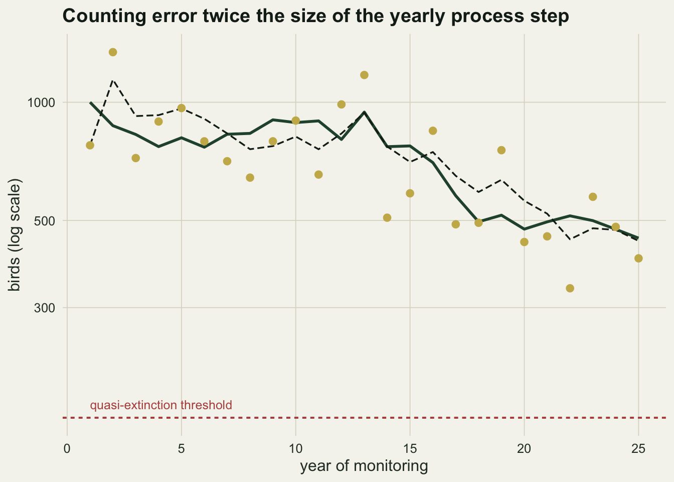
For this series the variance of the log differences is 14.0 times the true process variance. The true fifty-year risk, from the true drift, variance and final state, is 0.332; the naive risk is 0.843, and the state-space estimate is 0.554. One series proves nothing; the rest of the post counts.
The inflation is a closed form
The yearly change in the log count is y[t+1] - y[t] = mu + (process step) + e[t+1] - e[t]. The process step has variance sigma_p^2, and the two error terms add 2 sigma_o^2, so Var(y[t+1] - y[t]) = sigma_p^2 + 2 sigma_o^2. The error terms also make neighbouring differences negatively correlated, with covariance -sigma_o^2, and that changes the expectation of the sample variance over n = T - 1 differences slightly: working it through gives E[s^2] = sigma_p^2 + 2 sigma_o^2 (1 + 1/n). The drift estimate is barely touched, because the mean of the differences telescopes to (y[T] - y[1]) / n and only the first and last errors survive: its variance is sigma_p^2 / n + 2 sigma_o^2 / n^2. Holmes (2001) describes the same inflation as raising the line of var[ln(R[t + tau] / R[t])] against the lag tau while keeping its slope approximately the same, where R[t] is a running sum of L counts, and the slope method reads the process variance from that slope. The “approximately” matters at short lags. For lags up to L, the counting errors in the 2 tau counts that the two running sums do not share still grow with the lag, adding about 2 tau sigma_o^2 / L^2 on a linear approximation; and the paper reports that, even without counting error, the slope method underestimates the process variability by about 15 per cent at L = 4 in 100-year series, because R[t] is correlated with R[t + tau] and successive log ratios are serially correlated. The chunk below checks both expressions on 4000 series at each of nine error levels.
set.seed(43102)
cf_ratio <- seq(0, 2, by = 0.25)
cf_reps  <- 4000
cf_tab <- do.call(rbind, lapply(cf_ratio, function(r) {
  so <- r * sp_a
  steps <- matrix(rnorm(cf_reps * (n_a - 1), mu_a, sp_a), cf_reps)
  x_mat <- cbind(log(n_start), log(n_start) + t(apply(steps, 1, cumsum)))
  y_mat <- x_mat + matrix(rnorm(cf_reps * n_a, 0, so), cf_reps)
  d_mat <- y_mat[, -1] - y_mat[, -n_a]
  s2_vec <- apply(d_mat, 1, var)
  m_vec  <- rowMeans(d_mat)
  n_d <- n_a - 1
  data.frame(ratio = r, mean_s2 = mean(s2_vec), se_s2 = sd(s2_vec) / sqrt(cf_reps),
             q10 = quantile(s2_vec, 0.1) / sp_a^2, q50 = median(s2_vec) / sp_a^2,
             q90 = quantile(s2_vec, 0.9) / sp_a^2,
             pop_form = sp_a^2 + 2 * so^2,
             samp_form = sp_a^2 + 2 * so^2 * (1 + 1 / n_d),
             var_m = var(m_vec), var_m_form = sp_a^2 / n_d + 2 * so^2 / n_d^2)
}))
cf_z   <- (cf_tab$mean_s2 - cf_tab$samp_form) / cf_tab$se_s2
cf_dev <- max(abs(cf_tab$mean_s2 / cf_tab$samp_form - 1))
cf_vm  <- max(abs(cf_tab$var_m / cf_tab$var_m_form - 1))
cf_at2 <- cf_tab[cf_tab$ratio == 2, ]
Across the nine error levels the mean sample variance lies within 0.9 per cent of sigma_p^2 + 2 sigma_o^2 (1 + 1/n), the largest standardised gap being 1.6 Monte Carlo standard errors, and the variance of the drift estimate within 2.9 per cent of its formula. At sigma_o = 2 sigma_p the population variance of the differences is 9 times the process variance and the expected sample variance 9.33 times, against a simulated mean of 9.34 and a median of 8.98. This reproduces the closed form by simulation; nothing here is new.
ggplot(cf_tab, aes(ratio)) +
  geom_ribbon(aes(ymin = q10, ymax = q90), fill = te_gold, alpha = 0.35) +
  geom_line(aes(y = samp_form / sp_a^2), colour = te_forest, linewidth = 1) +
  geom_point(aes(y = mean_s2 / sp_a^2), colour = te_rust, size = 2.4) +
  labs(x = "counting error SD / process SD", y = "variance of log differences / process variance",
       title = "Twice the counting variance lands in the growth variance") +
  theme_datasheet()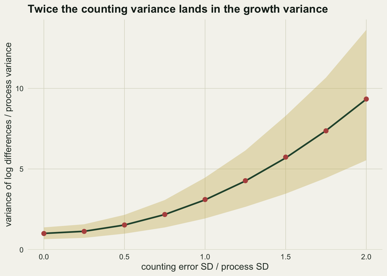
The band matters as much as the line. At sigma_o = 2 sigma_p the 10th to 90th percentile of the ratio runs from 5.5 to 13.6, so a single 25-year series gives only a rough reading of its own inflation, and any repair that subtracts a fixed amount inherits that spread.
The Dennis risk, and what counts as the truth
Before comparing estimates, the risk function itself is checked against a direct simulation of the Brownian motion it describes, on steps of one fiftieth of a year, for three combinations of drift and variance, including a positive drift, which several estimates below produce.
set.seed(43103)
ig_cases <- data.frame(mu = c(-0.01, -0.01, 0.01), s2 = c(0.01, 0.09, 0.09), xd = log(thr_frac))
ig_paths <- 4000
dt_step  <- 1 / 50
ig_tab <- do.call(rbind, lapply(seq_len(nrow(ig_cases)), function(i) {
  pos <- rep(ig_cases$xd[i], ig_paths)
  hit <- rep(FALSE, ig_paths)
  for (k in seq_len(horizon / dt_step)) {
    pos <- pos + rnorm(ig_paths, ig_cases$mu[i] * dt_step, sqrt(ig_cases$s2[i] * dt_step))
    hit <- hit | pos <= 0
  }
  data.frame(ig_cases[i, ], formula = risk_ig(ig_cases$mu[i], ig_cases$s2[i], ig_cases$xd[i]),
             simulated = mean(hit), se = sd(hit) / sqrt(ig_paths))
}))
ig_gap <- max(abs(ig_tab$formula - ig_tab$simulated) / ig_tab$se)
print(format(ig_tab, digits = 3), row.names = FALSE)
mu s2 xd formula simulated se
-0.01 0.01 1.61 0.094 0.0968 0.00467
-0.01 0.09 1.61 0.529 0.5215 0.00790
0.01 0.09 1.61 0.370 0.3590 0.00759The formula and the fine-step simulation agree to within 1.5 binomial standard errors in all three cases; a path watched only once a year misses some crossings between censuses, which is why the PVA post found its annual simulation running a little below the formula. That is a property of the census, not of the formula, and it is the same for every estimate here.
The truth for each series is the Dennis risk computed from the true drift, the true process variance and the true final log abundance, which the simulation knows and the warden does not. So the true risk is a per-series quantity: two series with the same parameters end at different sizes and carry different risks. Every comparison below is made series by series, the estimate against its own series’ truth.
Twenty-five years of counts
The first comparison is the point above, sigma_o = 2 sigma_p, over 2000 series.
summ_run <- function(res) {
  tr <- pmax(res[, "true"], 1e-4)
  meths <- c("naive", "naive_xt", "true_yd", "known", "holmes", "ss")
  data.frame(method = meths,
    med    = sapply(meths, function(k) median(res[, k])),
    q10    = sapply(meths, function(k) quantile(res[, k], 0.1)),
    q90    = sapply(meths, function(k) quantile(res[, k], 0.9)),
    over   = sapply(meths, function(k) mean(res[, k] > res[, "true"])),
    within = sapply(meths, function(k) mean(abs(log2(pmax(res[, k], 1e-4) / tr)) < 1)),
    abserr = sapply(meths, function(k) median(abs(res[, k] - res[, "true"]))),
    row.names = meths)
}
set.seed(43104)
res_25 <- t(replicate(2000, one_series(n_a, mu_a, sp_a, so_a)))
tab_25 <- summ_run(res_25)
true_25 <- quantile(res_25[, "true"], c(0.1, 0.5, 0.9))
fl_25 <- colMeans(res_25[, c("kn_floor", "ho_floor", "ss_floor")])
code_25 <- mean(res_25[, "ss_code"] != 0)
se_share <- function(p, n) sqrt(p * (1 - p) / n)
se_max_25 <- max(se_share(tab_25$within, nrow(res_25)))
kn_left <- 2 * so_a^2 / (n_a - 1) / sp_a^2
print(format(round(tab_25[, -1], 4), scientific = FALSE))
med q10 q90 over within abserr
naive 0.5409 0.1524 0.8828 0.9965 0.0875 0.3957
naive_xt 0.5353 0.1610 0.8726 0.9975 0.0745 0.4043
true_yd 0.0994 0.0106 0.4039 0.5105 0.7990 0.0294
known 0.1248 0.0000 0.9977 0.5565 0.1505 0.1328
holmes 0.1142 0.0000 0.9594 0.5295 0.2585 0.0812
ss 0.0902 0.0000 0.9513 0.5070 0.2495 0.0848The true fifty-year risk has a median of 0.093 over these series, with a 10th to 90th percentile of 0.012 to 0.376. The naive risk has a median of 0.541 (10th to 90th percentile 0.152 to 0.883) and is above its own series’ truth in 99.7 per cent of series. It lands within a factor of two of the truth in 8.8 per cent.
The distance to the threshold is not what does this. Measuring the naive distance from the true final state instead of the last count changes the median to 0.535 and the within-two share to 7.4 per cent; keeping the last count but using the true drift and variance gives a median of 0.099 and puts 79.9 per cent of series within a factor of two. The error in the last count costs something, but the overstatement is the variance.
The three repairs bring the median down to 0.125 for the known-error subtraction, 0.114 for the Holmes slope method and 0.090 for the state-space fit, against the true median of 0.093. Series by series they are poor. Within a factor of two of the truth: 15.0 per cent for the known-error repair, 25.9 per cent for Holmes and 24.9 per cent for the state-space fit (Monte Carlo standard error at most 0.010 on each share). Each is above the truth in 51 to 56 per cent of series, which is roughly half: they scatter on both sides of the truth rather than sitting above it.
Two of those medians are less clean than they look. By the expectation above, the known-error subtraction leaves 2 sigma_o^2 / n of counting variance in on average, 0.33 of the process variance here. The Holmes variance slope is off in both directions at once, and the chunk below separates the two by running the same method on the same kind of series counted without error.
set.seed(43107)
ho_exact <- replicate(2000, {
  x_ex <- cumsum(c(log(n_start), rnorm(n_a - 1, mu_a, sp_a)))
  holmes_fit(exp(x_ex))[["s2"]]
})
ho_r_exact  <- mean(ho_exact) / sp_a^2
ho_r_err    <- mean(res_25[, "ho_s2"]) / sp_a^2
ho_gap_se   <- sqrt(var(ho_exact) / length(ho_exact) +
                    var(res_25[, "ho_s2"]) / nrow(res_25)) / sp_a^2
ho_gap_form <- 2 * so_a^2 / run_len^2 / sp_a^2
Without counting error the Holmes variance averages 0.61 times the process variance over 2000 series of 25 years: below one, in the direction the paper reports without counting error, and further below one than its figure of about 15 per cent, which is for 100-year series. With the counting error of this section it averages 1.15 times. The gap, 0.54 (standard error 0.02), is close to the slope of 2 tau sigma_o^2 / L^2 against tau that the linear approximation above gives, 0.50 of the process variance. So the Holmes median sits near the true median partly because two biases offset each other at this point.
Part of the scatter is the variance floor. Subtracting the known error variance leaves nothing, or less than nothing, in 37.8 per cent of series, because the sample variance itself scatters as widely as the band in the figure above. The state-space fit puts the process variance on zero in 13.4 per cent, the counterpart of the observation variance on zero in the post on observation error estimated as zero; StructTS() reported a convergence code other than zero in 0.2 per cent of fits, which are kept. The Holmes variance slope reached the floor in 0 of the 2000 series, and its risk spreads widely all the same. A process variance at the floor turns the risk into a near certainty either way: close to one if the estimated drift carries the population across the threshold within the horizon, close to zero if it does not. Such series account for part of the rows of points along the top and the bottom of the next figure.
meth_lab <- c(naive = "naive", known = "known error subtracted", holmes = "Holmes slope method",
              ss = "state-space fit")
sc_df <- do.call(rbind, lapply(names(meth_lab), function(k)
  data.frame(method = meth_lab[[k]], true = pmax(res_25[, "true"], 1e-4),
             est = pmax(res_25[, k], 1e-4))))
sc_df$method <- factor(sc_df$method, meth_lab)
sc_lab <- data.frame(method = factor(meth_lab, meth_lab),
                     lab = sprintf("within 2x: %.0f%%", 100 * tab_25[names(meth_lab), "within"]))
sc_plot <- ggplot(sc_df, aes(true, est)) +
  geom_point(colour = te_forest, alpha = 0.25, size = 0.9) +
  geom_abline(slope = 1, intercept = 0, colour = te_ink, linewidth = 0.6) +
  geom_abline(slope = 1, intercept = c(-1, 1) * log10(2), colour = te_rust,
              linetype = "22", linewidth = 0.6) +
  geom_text(data = sc_lab, aes(x = 1.2e-4, y = 0.9, label = lab), hjust = 0, vjust = 1,
            size = 3.3, colour = te_ink) +
  facet_wrap(~ method, nrow = 2) +
  scale_x_log10(limits = c(1e-4, 1), breaks = c(1e-4, 1e-2, 1),
                labels = c("0.0001", "0.01", "1")) +
  scale_y_log10(limits = c(1e-4, 1), breaks = c(1e-4, 1e-3, 1e-2, 0.1, 1),
                labels = c("0.0001", "0.001", "0.01", "0.1", "1")) +
  coord_equal() +
  labs(x = "true risk of quasi-extinction in 50 years", y = "estimated risk",
       title = "The naive risk sits high; the repairs scatter") +
  theme_datasheet()
sc_plot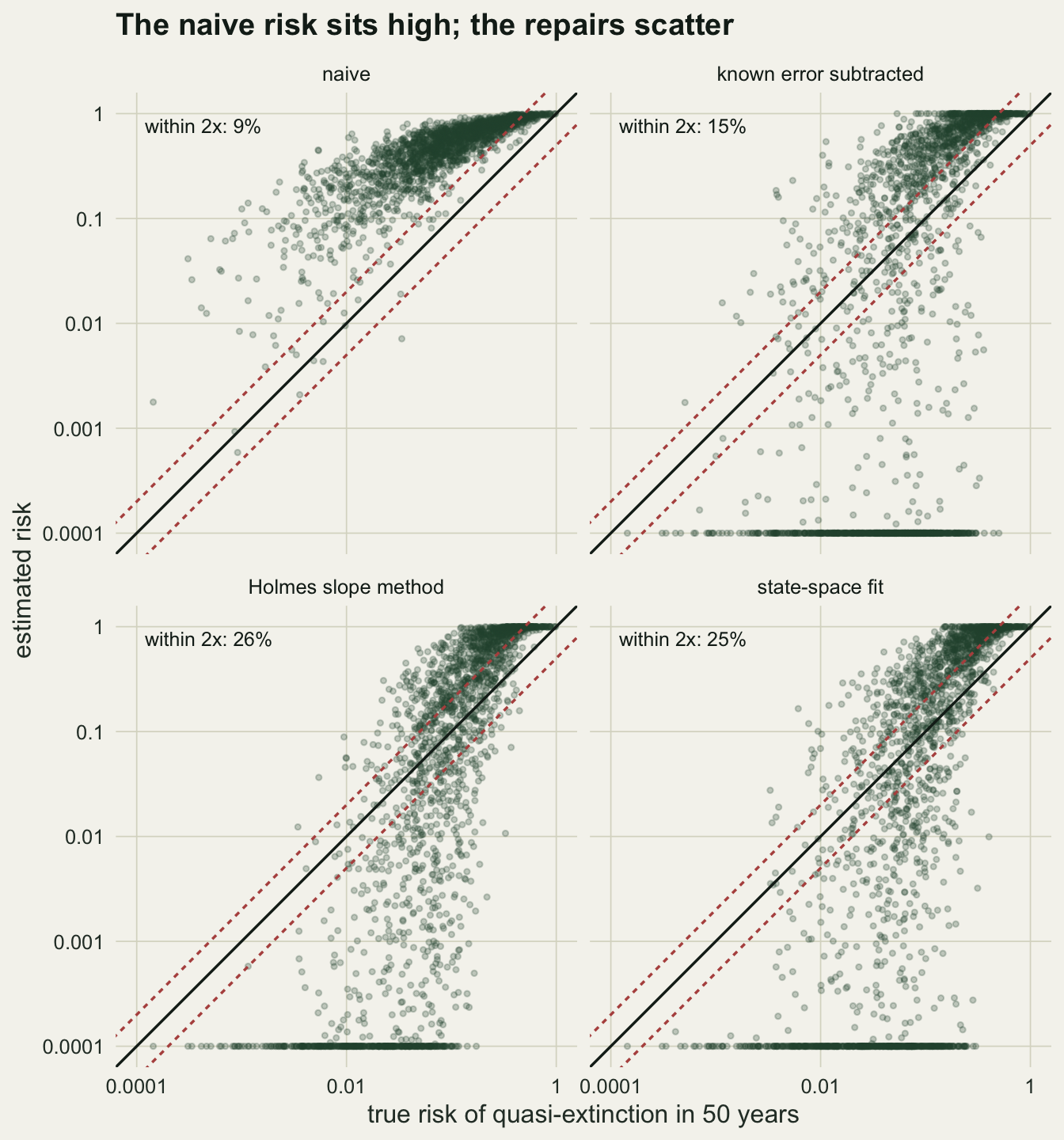
A longer series
The naive bias is not a small-sample effect: the variance it estimates is the wrong quantity, and a longer series only estimates the wrong quantity more precisely. The same point with a hundred years of counts, over 1000 series:
set.seed(43105)
res_100 <- t(replicate(1000, one_series(100, mu_a, sp_a, so_a)))
tab_100 <- summ_run(res_100)
true_100 <- quantile(res_100[, "true"], c(0.1, 0.5, 0.9))
fl_100 <- colMeans(res_100[, c("kn_floor", "ho_floor", "ss_floor")])
se_max_100 <- max(se_share(tab_100$within, nrow(res_100)))
print(format(round(tab_100[, -1], 4), scientific = FALSE))
med q10 q90 over within abserr
naive 0.5357 0.1436 0.9237 0.941 0.243 0.3221
naive_xt 0.5391 0.1565 0.9116 0.952 0.248 0.3336
true_yd 0.1011 0.0007 0.7885 0.455 0.803 0.0185
known 0.0680 0.0000 0.9794 0.503 0.435 0.0582
holmes 0.1332 0.0002 0.9334 0.574 0.690 0.0274
ss 0.1042 0.0000 0.9517 0.488 0.618 0.0276With a hundred years the true risk has a median of 0.102 (10th to 90th percentile 0.001 to 0.756, wider than before because the final state has had longer to wander). The naive median is 0.536, above the truth in 94.1 per cent of series and within a factor of two in 24.3 per cent. That share rises from the 25-year run while the naive median does not move, which goes with the wider spread of true risks: more of them sit high, where the inflated estimate lands. The repairs improve: within a factor of two in 43.5 per cent of series for the known-error subtraction, 69.0 per cent for Holmes and 61.8 per cent for the state-space fit (standard error at most 0.016). The known-error subtraction still hits the floor in 27.3 per cent of series, while the state-space fit does so in 0.2 per cent. Even at a century of counts, 31 per cent or more of series get a repaired risk more than a factor of two away from their own truth.
When the naive risk is no worse
The comparison so far used one parameter point with a low true risk and counting error twice the process noise. The grid below varies the ratio sigma_o / sigma_p from 0.5 to 2 at two parameter points and 25 years of counts: the one above, where the true risk is low, and a steeper, noisier decline (drift -0.02, process standard deviation 0.15) where the true risk is moderate. At each of the eight cells, 1000 series. Besides the within-two share, each cell records a paired measure: the share of series in which the naive risk is closer to the truth, in absolute probability, than a given repair. A share above one half means the naive estimate wins more series than it loses against that repair.
fam_tab <- data.frame(family = c("low true risk", "moderate true risk"),
                      mu = c(mu_a, -0.02), sp = c(sp_a, 0.15))
grid_ratio <- c(0.5, 1, 1.5, 2)
reps <- c("known", "holmes", "ss")
set.seed(43106)
grid_tab <- do.call(rbind, lapply(seq_len(nrow(fam_tab)), function(f)
  do.call(rbind, lapply(grid_ratio, function(r) {
    res <- t(replicate(1000, one_series(n_a, fam_tab$mu[f], fam_tab$sp[f], r * fam_tab$sp[f])))
    tb <- summ_run(res)
    err_n <- abs(res[, "naive"] - res[, "true"])
    tb$closer <- NA
    tb[reps, "closer"] <- sapply(reps, function(m) mean(err_n < abs(res[, m] - res[, "true"])))
    in_two <- function(k) abs(log2(pmax(res[, k], 1e-4) / pmax(res[, "true"], 1e-4))) < 1
    below <- res[, "true"] < 0.3
    tb$extreme <- sapply(rownames(tb), function(k) mean(res[, k] < 0.02 | res[, k] > 0.98))
    tb$within_below <- sapply(rownames(tb), function(k) mean(in_two(k)[below]))
    tb$n_below <- sum(below)
    tb$within_sp <- mean(in_two("naive_sp"))
    tb$extreme_sp <- mean(res[, "naive_sp"] < 0.02 | res[, "naive_sp"] > 0.98)
    tb$true_extreme <- mean(res[, "true"] < 0.02 | res[, "true"] > 0.98)
    tb$true_half <- mean(res[, "true"] >= 0.5)
    tb$wdiff_se <- NA
    tb[reps, "wdiff_se"] <- sapply(reps, function(m) sd(in_two("naive") - in_two(m)) / sqrt(nrow(res)))
    cbind(family = fam_tab$family[f], ratio = r, method = rownames(tb), tb[, -1],
          true_med = median(res[, "true"]), n_rep = nrow(res))
  }))))
rownames(grid_tab) <- NULL
gv <- function(fam, r, m, v) grid_tab[grid_tab$family == fam & grid_tab$ratio == r &
                                        grid_tab$method == m, v]
lo <- fam_tab$family[1]
mo <- fam_tab$family[2]
wide <- function(v) {
  out <- sapply(c("naive", reps), function(m) sapply(fam_tab$family, function(fm)
    sapply(grid_ratio, function(r) gv(fm, r, m, v))))
  data.frame(family = rep(fam_tab$family, each = length(grid_ratio)),
             ratio = grid_ratio, out, row.names = NULL)
}
print(format(wide("within"), digits = 3), row.names = FALSE)
family ratio naive known holmes ss
low true risk 0.5 0.313 0.270 0.216 0.293
low true risk 1.0 0.260 0.249 0.236 0.287
low true risk 1.5 0.130 0.203 0.238 0.271
low true risk 2.0 0.085 0.161 0.249 0.225
moderate true risk 0.5 0.739 0.644 0.532 0.598
moderate true risk 1.0 0.893 0.648 0.555 0.633
moderate true risk 1.5 0.807 0.580 0.553 0.587
moderate true risk 2.0 0.704 0.579 0.581 0.586print(format(wide("closer")[, c("family", "ratio", reps)], digits = 3), row.names = FALSE) family ratio known holmes ss
low true risk 0.5 0.636 0.669 0.503
low true risk 1.0 0.452 0.448 0.325
low true risk 1.5 0.232 0.258 0.204
low true risk 2.0 0.183 0.174 0.155
moderate true risk 0.5 0.799 0.790 0.629
moderate true risk 1.0 0.674 0.740 0.586
moderate true risk 1.5 0.598 0.556 0.517
moderate true risk 2.0 0.528 0.470 0.458best_rep <- function(fam, r) max(sapply(reps, function(m) gv(fam, r, m, "within")))
over_ge1 <- grid_tab[grid_tab$method == "naive" & grid_tab$ratio >= 1, "over"]
se_max_grid <- max(se_share(c(grid_tab$within, grid_tab$closer[!is.na(grid_tab$closer)]), 1000))
lo_max <- max(grid_tab$within[grid_tab$family == lo & grid_tab$method %in% c("naive", reps)])
mo_naive_best <- all(sapply(grid_ratio, function(r) gv(mo, r, "naive", "within") > best_rep(mo, r)))
stopifnot(mo_naive_best, best_rep(lo, 1) == gv(lo, 1, "ss", "within"))
se_below <- max(se_share(grid_tab[grid_tab$family == mo & grid_tab$ratio == 1 &
grid_tab$method %in% c("naive", "holmes", "ss"), "within_below"],
gv(mo, 1, "naive", "n_below")))rg_top <- grid_tab[grid_tab$method %in% names(meth_lab), c("family", "ratio", "method", "within")]
names(rg_top)[4] <- "share"
rg_top$panel <- "within 2x"
rg_bot <- grid_tab[grid_tab$method %in% reps, c("family", "ratio", "method", "closer")]
names(rg_bot)[4] <- "share"
rg_bot$panel <- "naive closer"
rg_df <- rbind(rg_top, rg_bot)
rg_df$method <- factor(meth_lab[rg_df$method], meth_lab)
rg_df$panel <- factor(rg_df$panel, c("within 2x", "naive closer"))
fam_med <- tapply(grid_tab$true_med, grid_tab$family, median)[fam_tab$family]
rg_df$family <- factor(rg_df$family, fam_tab$family,
sprintf("%s (median %.2f)", fam_tab$family, fam_med))
half_df <- data.frame(panel = factor("naive closer", levels(rg_df$panel)), y = 0.5)
ggplot(rg_df, aes(ratio, share, colour = method)) +
geom_hline(data = half_df, aes(yintercept = y), colour = te_body, linetype = "22",
linewidth = 0.5) +
geom_line(linewidth = 0.9) +
geom_point(size = 2.2) +
facet_grid(panel ~ family) +
scale_colour_manual(values = c(te_rust, te_gold, te_ink, te_forest), name = NULL) +
scale_y_continuous(limits = c(0, 1)) +
labs(x = "counting error SD / process SD", y = "share of series",
title = "Where the truth sits decides whether the bias hurts") +
theme_datasheet() +
theme(legend.position = "bottom") +
guides(colour = guide_legend(nrow = 2))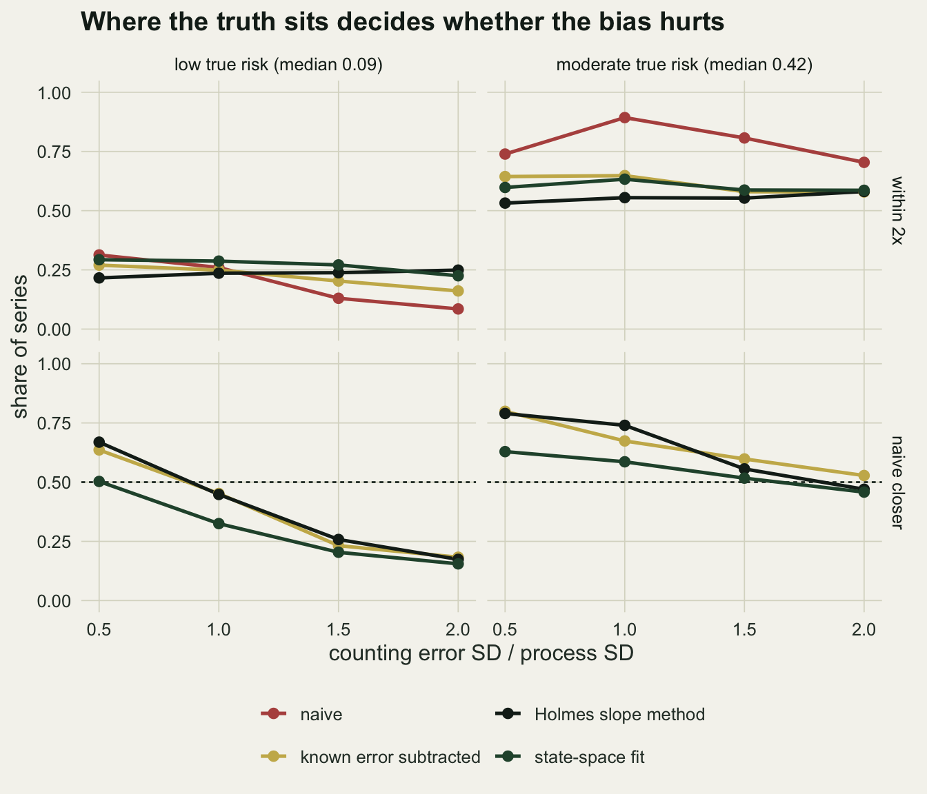
In the low-risk family, at sigma_o = sigma_p / 2, the naive estimate is within a factor of two in 31.3 per cent of series against 29.3 per cent for the best repair, and it is closer to the truth than the state-space fit in 50.3 per cent of series: no worse. At sigma_o = sigma_p the within-two shares are 26.0 per cent for the naive estimate and 28.7 for the state-space fit, the best repair here, a gap of 1.5 standard errors of the paired difference, so no clear winner; but the paired measure has turned: the naive risk is closer than the state-space fit in only 32.5 per cent of series, because on the probability scale its overshoot is large where the truth is small. At 2 sigma_p the naive within-two share is 8.5 per cent and it is closer than the state-space fit in 15.5 per cent. The highest within-two share anywhere in this family, over all four estimates, is 31.3 per cent.
In the moderate-risk family the naive estimate has the highest within-two share of the four at every ratio in the grid, including sigma_o = 2 sigma_p, where it is 70.4 per cent against 58.6 per cent for the best repair. On the paired measure it beats the state-space fit in 62.9 per cent of series at sigma_o = sigma_p / 2 and 58.6 per cent at sigma_o = sigma_p, and falls slightly behind it by 2 sigma_p (45.8 per cent). It is still biased: above the truth in 94.7 per cent of series at 2 sigma_p.
Part of this is the yardstick: for a series whose true risk is one half or more, any overestimate is within a factor of two, and 39.2 per cent of the series in the moderate-risk cell at sigma_o = sigma_p have a true risk that high. That is not the main reason. Among the 338 series of that cell whose true risk is below 0.3, the naive estimate is still within a factor of two in 71.0 per cent, against 18.0 per cent for the state-space fit and 12.4 per cent for Holmes (standard error at most 0.025). The weak ingredient is the drift, which 25 counts pin down only loosely, as the PVA post notes. In the same cell the true drift and variance with the observed distance put 99.4 per cent of series within a factor of two; the estimated drift with the true process variance puts only 66.5 per cent there, and the estimated drift with the inflated variance, the naive estimate, 89.3 per cent. A smaller variance turns an error in the drift into a risk nearer zero or one: 38.1 per cent of state-space risks and 47.4 per cent of Holmes risks fall below 0.02 or above 0.98, and 33.5 per cent of risks from the estimated drift with the true variance, against 11.8 per cent of naive risks and 2.2 per cent of true risks. The inflated variance helps by accident; its bias shows most where the true risk is far from where it pushes the estimate, as in the low-risk family.
So the regime is set by two things together, the size of the counting error against the process noise and where the true risk lies, and the naive fit reveals neither. What holds in all six cells with sigma_o at or above sigma_p is the direction: the naive risk is above the true risk in 76.1 to 99.4 per cent of series (Monte Carlo standard error at most 0.016 on any share in the grid).
What to report
State the survey method and what is known about its repeatability. If replicate counts exist, estimate sigma_o from them and report it next to the square root of the naive variance of the log differences; the closed form says how much of that variance is counting error, and if 2 sigma_o^2 is a large share of it, the naive risk is very likely above the truth, and several times the truth when that truth is small.
Report a repaired estimate next to the naive one, not instead of it, and say which repair: the subtraction needs sigma_o from outside the series; the Holmes slope method needs a running-sum window and a range of lags, both of which are choices; the state-space fit estimates everything from the series and can put the process variance on zero. Report whether a variance landed on zero, because a risk computed from a zero process variance is close to zero or one by construction.
Report an interval, never a single risk. With 25 years of counts at the low-risk point the repairs above were within a factor of two of the truth in a minority of series, even with the right model. The PVA post’s bootstrap already gives a wide interval with exact counts; with counting error the interval also has to carry the uncertainty in how the variance is split between process and counting, and a parametric bootstrap of the fitted state-space model is the natural way to get it (not run here).
If the risk is used to rank populations, the naive estimate ranks them by their counting error as much as by their dynamics: a well-counted population and a badly counted one with the same true risk get different naive risks.
Honest limits
The process is a density-independent random walk, and the counting error is lognormal, independent between years and constant in size. Real survey error often grows as a population thins out, is correlated between years when the same observer or method is used, and on count data is Poisson or negative binomial rather than lognormal; none of that was simulated.
The true risk is the diffusion risk from the true parameters and state, which is the quantity every estimate here aims at; it is not the risk of an annual census, which runs a little lower, and not the risk for a finite population with demographic stochasticity.
The known-error repair is given the exact sigma_o. With a handful of replicate counts sigma_o is itself uncertain, and the repair can only do worse than shown.
The Holmes method was run with one window length and one set of lags; other choices change its variance and its floor behaviour, and the comparison with the other repairs holds for these choices only. At these choices its variance runs low without counting error and carries part of the counting error in its slope, and the two offset each other at the main point of the post; at another error level or window they will not offset in the same way. The paper’s own risk measures are for a proportional decline from the current size, not for an absolute threshold; the use of the last running sum as the current size is a choice made here.
The state-space fit uses StructTS() maximum likelihood with its default diffuse start, one optimiser run per series; fits with a nonzero convergence code were kept, and a restricted likelihood fit as in Staples and colleagues (2004), or several starts, may put fewer process variances on zero.
The regime result rests on two parameter points and one horizon. The claim that the naive estimate does no worse where the true risk is moderate is about the within-two share and the paired closer share at those points, not a general rule; a different threshold or horizon moves the truth and so moves the comparison.
References
Dennis B, Munholland PL, Scott JM 1991 Ecological Monographs 61(2):115-143 (10.2307/1943004)
Holmes EE 2001 Proceedings of the National Academy of Sciences 98(9):5072-5077 (10.1073/pnas.081055898)
Staples DF, Taper ML, Dennis B 2004 Ecology 85(4):923-929 (10.1890/03-3101)