library(ggplot2)

te_pal <- list(forest = "#275139", green = "#2f8f63", sage = "#93a87f",
               clay = "#b5534e", gold = "#cda23f", line = "#dad9ca",
               ink = "#16241d", paper = "#f5f4ee")

theme_te <- function() {
  theme_minimal(base_size = 12) +
    theme(panel.grid.minor = element_blank(),
          panel.grid.major = element_line(colour = "#e7e6dc"),
          plot.background = element_rect(fill = "#f5f4ee", colour = NA),
          panel.background = element_rect(fill = "#f5f4ee", colour = NA),
          plot.title = element_text(face = "bold", colour = te_pal$ink),
          axis.title = element_text(colour = "#2c3a31"),
          axis.text = element_text(colour = "#2c3a31"),
          legend.position = "bottom")
}The price of harmonising a species list
R
monitoring
data cleaning
ecology tutorial
Pushing two decades of records onto one taxonomic backbone destroys information. Measuring the cost: hidden trends, lost richness and a silent trait join.
A grassland scheme has twenty years of counts from four permanent plots. The first ten years were recorded by someone using a regional flora from the 1990s; the last ten by someone using the current national checklist. Between the two, a revision moved a genus, lumped two segregates and split an aggregate into three. Before anything can be plotted, the two halves have to be brought onto one list of names, and the standard advice is to take everything to the newest backbone.
That instruction sounds like tidying, and it is not. Harmonisation is a many-to-one map applied to data, and a many-to-one map destroys information. What it destroys is sometimes exactly the thing the monitoring scheme exists to detect, and the damage does not appear where anyone is looking for it: the code runs, nothing warns, and the summary table looks better than before.
This post is the second half of a pair. Taxonomic revision and species trends measures the phenomenon: what a revision does to an apparent trend when the analysis simply carries on. This post measures the price of the repair. It is also a different bill from Cleaning species names before you count, which pays for spelling: stray whitespace, four capitalisations of one epithet, a lookup table that collapses them. That post closes by calling name resolution a decision to be written down rather than a function to be called. Here the decision gets a number attached to it.
Six measurements follow, all on synthetic data with the generating truth known, so every error is a difference from a value we set rather than an argument about what should have happened. Two segregates with opposite trends get lumped and the aggregate is regressed, then the trend contrast is swept to find where the declining member stops being visible. A whole flora is aggregated to the coarsest concept both authorities accept. A trait table keyed on the old names is joined to a community matrix keyed on the new ones. And the same analysis is run under two backbone versions that differ in a handful of taxa. The post then returns to the era break it opened with, and measures three ways of handling it against the known truth.
One constraint on the code: no taxonomic package is used. taxize, rgbif and WorldFlora all do real work against real authorities, and their calls appear once below in a block that never runs. Everything measured here uses hand-built lookup tables, which is the more honest representation anyway. A backbone is a table. It has a version, an author and a set of decisions in it, and treating it as a fact rather than as data is where the trouble starts.
A backbone is a table with two columns you care about
Take twelve names as they appear on the recording cards, and two authorities: a 2005 list and a 2024 list. Each authority maps every recorded name to an accepted name. The two maps do not agree, and the disagreements come in three flavours. A pair of segregates accepted separately in 2005 is lumped in 2024. An aggregate accepted as one entity in 2005 is split in 2024. A species keeps its circumscription but changes genus, so the string changes while nothing biological does.
crosswalk <- data.frame(
  recorded  = c("Festuca ovina", "Festuca guestfalica", "Festuca lemanii",
                "Alchemilla vulgaris", "Alchemilla monticola",
                "Alchemilla glabra", "Carex viridula", "Carex oederi",
                "Carex demissa", "Hieracium pilosella", "Thymus pulegioides",
                "Briza media"),
  name_2005 = c("Festuca ovina", "Festuca guestfalica", "Festuca lemanii",
                "Alchemilla vulgaris", "Alchemilla vulgaris",
                "Alchemilla glabra", "Carex viridula", "Carex viridula",
                "Carex viridula", "Hieracium pilosella", "Thymus pulegioides",
                "Briza media"),
  name_2024 = c("Festuca ovina", "Festuca ovina", "Festuca lemanii",
                "Alchemilla vulgaris", "Alchemilla monticola",
                "Alchemilla glabra", "Carex viridula", "Carex oederi",
                "Carex demissa", "Pilosella officinarum", "Thymus pulegioides",
                "Briza media"),
  stringsAsFactors = FALSE)

print(crosswalk[, c("recorded", "name_2005", "name_2024")])
recorded name_2005 name_2024
1 Festuca ovina Festuca ovina Festuca ovina
2 Festuca guestfalica Festuca guestfalica Festuca ovina
3 Festuca lemanii Festuca lemanii Festuca lemanii
4 Alchemilla vulgaris Alchemilla vulgaris Alchemilla vulgaris
5 Alchemilla monticola Alchemilla vulgaris Alchemilla monticola
6 Alchemilla glabra Alchemilla glabra Alchemilla glabra
7 Carex viridula Carex viridula Carex viridula
8 Carex oederi Carex viridula Carex oederi
9 Carex demissa Carex viridula Carex demissa
10 Hieracium pilosella Hieracium pilosella Pilosella officinarum
11 Thymus pulegioides Thymus pulegioides Thymus pulegioides
12 Briza media Briza media Briza mediaA third route, the safe one, is to refuse both authorities and work at the coarsest grouping they both agree on, and that grouping is not something you choose by eye. Two recorded names belong to the same coarsest common concept if either authority puts them under one accepted name, and the relation is transitive: if 2005 joins A to B and 2024 joins B to C, then A, B and C are one concept whether you like it or not. That is a connected-components problem, and a short union-find in base R solves it.
common_concept <- function(a, b) {
  parent <- seq_along(a)
  find <- function(i) {
    while (parent[i] != i) i <- parent[i]
    i
  }
  unite <- function(i, j) {
    ri <- find(i)
    rj <- find(j)
    if (ri != rj) parent[rj] <<- ri
  }
  for (key in list(a, b)) {
    for (g in split(seq_along(a), key)) {
      if (length(g) > 1) for (k in g[-1]) unite(g[1], k)
    }
  }
  root <- vapply(seq_along(a), find, integer(1))
  lab <- vapply(split(seq_along(a), root), function(g) {
    cand <- c(b[g], a[g])
    cover <- vapply(cand, function(nm) sum(a[g] == nm | b[g] == nm), numeric(1))
    paste0(cand[which.max(cover)], if (length(g) > 1) " agg." else "")
  }, character(1))
  unname(lab[as.character(root)])
}

crosswalk$concept <- common_concept(crosswalk$name_2005, crosswalk$name_2024)
print(unique(crosswalk[, c("name_2005", "name_2024", "concept")]))
name_2005 name_2024 concept
1 Festuca ovina Festuca ovina Festuca ovina agg.
2 Festuca guestfalica Festuca ovina Festuca ovina agg.
3 Festuca lemanii Festuca lemanii Festuca lemanii
4 Alchemilla vulgaris Alchemilla vulgaris Alchemilla vulgaris agg.
5 Alchemilla vulgaris Alchemilla monticola Alchemilla vulgaris agg.
6 Alchemilla glabra Alchemilla glabra Alchemilla glabra
7 Carex viridula Carex viridula Carex viridula agg.
8 Carex viridula Carex oederi Carex viridula agg.
9 Carex viridula Carex demissa Carex viridula agg.
10 Hieracium pilosella Pilosella officinarum Pilosella officinarum
11 Thymus pulegioides Thymus pulegioides Thymus pulegioides
12 Briza media Briza media Briza median_rec <- nrow(crosswalk)
n_05 <- length(unique(crosswalk$name_2005))
n_24 <- length(unique(crosswalk$name_2024))
n_cc <- length(unique(crosswalk$concept))
print(c(recorded_names = n_rec, accepted_2005 = n_05,
accepted_2024 = n_24, common_concepts = n_cc)) recorded_names accepted_2005 accepted_2024 common_concepts
12 9 11 8 The twelve cards resolve to 9 accepted names under the 2005 authority and 11 under the 2024 one. The coarsest grouping both authorities can live with has 8 entities in it, fewer than either, which is the first thing worth saying out loud: the safe route is coarser than either backbone rather than a compromise between them. Refusing to choose costs 3 entities against the current list and 1 against the old one.
For reference, the calls that would do this against a real authority look like the block below. It is not run here.
# taxize::gnr_resolve(sci = crosswalk$recorded, data_source_ids = 11)
# rgbif::name_backbone_checklist(crosswalk$recorded)
# WorldFlora::WFO.match(spec.data = crosswalk$recorded, WFO.data = wfo)
Each of those returns a table with a match, a match type and a confidence score, and each is versioned: the GBIF backbone is rebuilt periodically, World Flora Online has dated releases. Grenie et al. (2023) compare the available tools and databases and find that they disagree with each other on a non-trivial share of names, which is the reason the version belongs in the methods section.
Two segregates, opposite trends, one accepted name
Now the measurement that matters most. Festuca ovina in the strict sense and Festuca guestfalica were accepted separately in 2005 and are one name in 2024. Suppose the strict species is increasing and the segregate is declining at a similar rate. What does the aggregate do? The counts below are Poisson with a log-linear trend, centred on the middle of the survey so the two species have the same expected abundance there. Both trends are set explicitly: b_ovina is 0.055 and b_guest is -0.048 on the log scale per year.
set.seed(20260803)
yr <- 2005:2024
t_c <- yr - mean(yr)
m_mid <- 42
b_ovina <- 0.055
b_guest <- -0.048
cnt_ov <- rpois(length(yr), m_mid * exp(b_ovina * t_c))
cnt_gu <- rpois(length(yr), m_mid * exp(b_guest * t_c))
cnt_ag <- cnt_ov + cnt_gu

fit_trend <- function(y) {
  m <- glm(y ~ t_c, family = poisson)
  s <- summary(m)$coefficients
  c(slope = unname(s[2, 1]), se = unname(s[2, 2]),
    lo = unname(s[2, 1] - qnorm(0.975) * s[2, 2]),
    hi = unname(s[2, 1] + qnorm(0.975) * s[2, 2]),
    p = unname(s[2, 4]))
}

tr <- rbind("Festuca ovina s.str." = fit_trend(cnt_ov),
            "Festuca guestfalica" = fit_trend(cnt_gu),
            "Festuca ovina agg." = fit_trend(cnt_ag))
pct <- 100 * (exp(tr[, c("slope", "lo", "hi")]) - 1)
print(round(tr, 5))
slope se lo hi p
Festuca ovina s.str. 0.05804 0.00607 0.04614 0.06993 0.00000
Festuca guestfalica -0.04767 0.00610 -0.05963 -0.03571 0.00000
Festuca ovina agg. 0.00572 0.00419 -0.00249 0.01393 0.17184print(round(pct, 3)) slope lo hi
Festuca ovina s.str. 5.975 4.722 7.244
Festuca guestfalica -4.655 -5.789 -3.508
Festuca ovina agg. 0.574 -0.248 1.402print(round(c(first_year_total = cnt_ag[1], last_year_total = cnt_ag[20],
ovina_fold_change = exp(tr[1, "slope"] * 19),
guest_fold_change = exp(tr[2, "slope"] * 19),
agg_fold_change = exp(tr[3, "slope"] * 19)), 4)) first_year_total last_year_total ovina_fold_change guest_fold_change
76.0000 100.0000 3.0123 0.4042
agg_fold_change
1.1148 Fitted separately, the two members are unambiguous. The strict species gains 5.975 per cent a year, a factor of 3.0123 over nineteen years, interval 4.722 to 7.244 per cent. The segregate loses 4.655 per cent a year and ends at 0.4042 of where it started, interval -5.789 to -3.508 per cent.
Add them together, as the 2024 backbone requires, and the aggregate gains 0.574 per cent a year with a p value of 0.1718 and an interval from -0.248 to 1.402 per cent, which contains zero. The correct report for the harmonised data is that Festuca ovina in the current sense shows no detectable change over twenty years. Both real trends are gone, and nothing in the output hints that there were two of them.
lab_seg <- c("Festuca ovina s.str.", "Festuca guestfalica",
             "Festuca ovina agg. (2024)")
seg_dat <- data.frame(
  year = rep(yr, 3),
  count = c(cnt_ov, cnt_gu, cnt_ag),
  series = factor(rep(lab_seg, each = length(yr)), levels = lab_seg))
cf_ag <- coef(glm(cnt_ag ~ t_c, family = poisson))
agg_line <- data.frame(year = yr, fit = exp(cf_ag[1] + cf_ag[2] * t_c))

ggplot(seg_dat, aes(year, count, colour = series)) +
  geom_line(linewidth = 0.7) +
  geom_point(size = 1.8) +
  geom_line(data = agg_line, aes(year, fit), inherit.aes = FALSE,
            colour = te_pal$ink, linetype = "22", linewidth = 0.8) +
  scale_colour_manual(values = c(te_pal$green, te_pal$clay, te_pal$ink),
                      name = NULL) +
  guides(colour = guide_legend(nrow = 2)) +
  labs(x = "year", y = "count in four plots",
       title = "Two trends, one accepted name") +
  theme_te() +
  theme(plot.margin = margin(8, 14, 4, 8))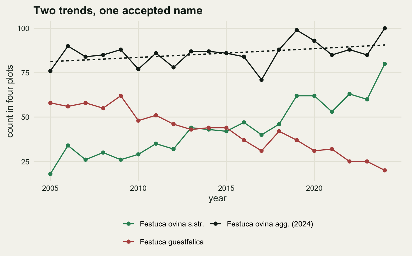
The dashed line is the aggregate’s fitted trend. It sits almost flat over a series that is not flat at all: the sum of a rising exponential and a falling one is a shallow U, and a log-linear model reads a shallow U as no change. The aggregate did not average the two signals into something intermediate. It converted them into an absence of signal.
How steep the loss has to be before the aggregate notices
That was one pair of trends. How large does the contrast have to be before the aggregate series recovers the decline? Hold the increasing member at b_ovina, sweep the declining member’s trend across a range, and at each value simulate n_rep twenty-year series, fitting a Poisson trend to the segregate alone and to the aggregate. glm.fit replaces glm because the sweep runs a few thousand fits and the formula machinery is most of the cost; the standard error comes from the inverse of the weighted cross-product matrix, which is what glm computes anyway.
set.seed(20260804)
Xd <- cbind(1, t_c)

slope_z <- function(y) {
  f <- glm.fit(Xd, y, family = poisson())
  b <- unname(f$coefficients[2])
  V <- solve(t(Xd) %*% (Xd * f$fitted.values))
  c(b, b / sqrt(V[2, 2]))
}

b_seq <- seq(-0.12, 0.01, by = 0.01)
n_rep <- 400
z_crit <- qnorm(0.975)
thr_hi <- 0.8
thr_lo <- 0.05
sweep_res <- do.call(rbind, lapply(b_seq, function(bg) {
  hit_agg <- 0
  hit_own <- 0
  sl <- numeric(n_rep)
  for (r in seq_len(n_rep)) {
    yo <- rpois(length(yr), m_mid * exp(b_ovina * t_c))
    yg <- rpois(length(yr), m_mid * exp(bg * t_c))
    sa <- slope_z(yo + yg)
    sg <- slope_z(yg)
    sl[r] <- sa[1]
    if (sa[2] < -z_crit) hit_agg <- hit_agg + 1
    if (sg[2] < -z_crit) hit_own <- hit_own + 1
  }
  data.frame(b_guest = bg, agg_slope = mean(sl),
             agg_detect = hit_agg / n_rep, own_detect = hit_own / n_rep)
}))
print(round(sweep_res, 4))
b_guest agg_slope agg_detect own_detect
1 -0.12 -0.0358 1.0000 1.0000
2 -0.11 -0.0296 1.0000 1.0000
3 -0.10 -0.0240 1.0000 1.0000
4 -0.09 -0.0188 0.9950 1.0000
5 -0.08 -0.0133 0.8950 1.0000
6 -0.07 -0.0077 0.4450 1.0000
7 -0.06 -0.0023 0.0700 1.0000
8 -0.05 0.0023 0.0025 1.0000
9 -0.04 0.0077 0.0000 1.0000
10 -0.03 0.0129 0.0000 1.0000
11 -0.02 0.0181 0.0000 0.8800
12 -0.01 0.0229 0.0000 0.3925
13 0.00 0.0279 0.0000 0.0250
14 0.01 0.0325 0.0000 0.0000least_steep <- function(v) sweep_res$b_guest[max(which(v >= thr_hi))]
b_own80 <- least_steep(sweep_res$own_detect)
b_agg80 <- least_steep(sweep_res$agg_detect)
blind <- sweep_res[sweep_res$own_detect >= thr_hi & sweep_res$agg_detect <= thr_lo, ]
print(round(c(n_replicates = n_rep, own_threshold = b_own80,
agg_threshold = b_agg80, ratio = b_agg80 / b_own80), 4)) n_replicates own_threshold agg_threshold ratio
400.00 -0.02 -0.08 4.00 print(round(c(blind_window_from = max(blind$b_guest),
blind_window_to = min(blind$b_guest),
blind_window_rows = nrow(blind)), 4))blind_window_from blind_window_to blind_window_rows
-0.02 -0.05 4.00 The declining segregate needs a trend of -0.02 on the log scale, about 1.98 per cent a year, before its own twenty-year series detects the decline four times in five. The aggregate needs -0.08, about 7.688 per cent a year, which is 4 times steeper.
Between those two thresholds is a window where the segregate’s decline is certain and the aggregate is silent. Across 4 of the swept values, from -0.02 down to -0.05, the segregate’s own series flags the decline in at least 80 per cent of replicates while the aggregate flags it in at most 5 per cent. At a trend of -0.05 the aggregate’s mean fitted slope is 0.00234, a positive number: the harmonised series reports a slight increase for a taxon one of whose two members is losing 4.877 per cent of its abundance every year.
lab_det <- c("segregate analysed on its own", "aggregate under the 2024 name")
det_dat <- data.frame(
  b_guest = rep(sweep_res$b_guest, 2),
  detect = c(sweep_res$own_detect, sweep_res$agg_detect),
  series = factor(rep(lab_det, each = nrow(sweep_res)), levels = lab_det))
band <- data.frame(xmin = min(blind$b_guest), xmax = max(blind$b_guest),
                   ymin = 0, ymax = 1)

ggplot(det_dat, aes(b_guest, detect, colour = series, shape = series)) +
  geom_rect(data = band, aes(xmin = xmin, xmax = xmax, ymin = ymin, ymax = ymax),
            inherit.aes = FALSE, fill = te_pal$sage, alpha = 0.25) +
  geom_line(linewidth = 0.7) +
  geom_point(size = 2.1) +
  scale_colour_manual(values = c(te_pal$forest, te_pal$clay), name = NULL) +
  scale_shape_manual(values = c(16, 17), name = NULL) +
  labs(x = "true log-scale trend of the declining segregate",
       y = "probability of detecting a decline",
       title = "What the aggregate can and cannot see") +
  theme_te() +
  theme(plot.margin = margin(8, 14, 4, 8))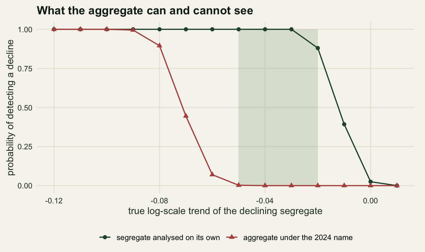
The shaded band is the blind window. Everything inside it is a real, steady, twenty-year decline that the segregate’s own counts would report with near certainty and that the harmonised aggregate reports as nothing at all. Isaac, Mallet and Mace (2004) argued that taxonomic inflation distorts macroecological patterns because species counts are not stable units; this is the same instability seen from the other end, where deflation removes the unit whose trajectory was the finding.
A whole flora, and what the safe route costs
The two-species case is clean because it was built to be. A real scheme has dozens of taxa, only some of which are contested, so the question becomes what aggregation costs on average rather than in the worst case. The flora below is built from families of one, two or three closely related entities, and each backbone decides independently whether to lump each family, with the 2005 list lumping more often than the 2024 one. A few concepts also get a new name in 2024 without any change of circumscription, standing in for genus transfers. Names are synthetic labels rather than binomials, which keeps the bookkeeping visible; a label is shared between the two backbones exactly when the accepted name did not change.
tag <- function(i) paste0("taxon_", formatC(i, width = 3, flag = "0"))

set.seed(20260805)
fam <- rep(seq_len(45), rep(c(1, 2, 3), times = c(20, 15, 10)))
n_tx <- length(fam)

build_backbone <- function(fid, p_lump) {
  out <- character(length(fid))
  for (g in split(seq_along(fid), fid)) {
    if (length(g) > 1 && runif(1) < p_lump) out[g] <- tag(min(g)) else out[g] <- tag(g)
  }
  out
}

nm05 <- build_backbone(fam, 0.60)
nm24 <- build_backbone(fam, 0.40)
moved <- sort(sample(which(!duplicated(nm24)), 6))
for (i in moved) nm24[nm24 == nm24[i]] <- paste0("taxon_", 200 + i)
cc <- common_concept(nm05, nm24)

membership <- function(key) {
  vapply(seq_along(key), function(i) paste(which(key == key[i]), collapse = ","),
         character(1))
}
n_disagree <- sum(membership(nm05) != membership(nm24))
print(c(recorded = n_tx, accepted_2005 = length(unique(nm05)),
        accepted_2024 = length(unique(nm24)),
        common_concepts = length(unique(cc)),
        circumscription_disagreements = n_disagree, renamed = length(moved)))
recorded accepted_2005
80 60
accepted_2024 common_concepts
69 53
circumscription_disagreements renamed
39 6 Of 80 recorded names, 39 sit in a group whose membership differs between the two authorities. Separately, 6 accepted concepts were given a new string in 2024 with no change of circumscription; the two sets overlap rather than adding up, because a concept can be both renamed and circumscribed differently. The 2005 list has 60 accepted names, the 2024 list 69, and the coarsest common concept 53.
Counts come next: four plots, twenty annual visits, a per-taxon intercept and a per-taxon log-linear trend drawn from a distribution whose mean is slightly negative, so the flora as a whole is thinning. Nothing about the trends is tied to the naming, which matters: any attenuation measured below comes from aggregation arithmetic and not from a rigged correlation between a taxon’s trend and whether it happens to be contested.
n_plot <- 4
pt <- expand.grid(year = yr, plot = seq_len(n_plot))
pt$t_c <- pt$year - mean(yr)
a_i <- rnorm(n_tx, log(0.9), 1.1)
b_i <- rnorm(n_tx, -0.025, 0.045)
pl_eff <- rnorm(n_plot, 0, 0.3)
lam <- exp(outer(a_i, rep(1, nrow(pt))) + outer(b_i, pt$t_c) +
             outer(rep(1, n_tx), pl_eff[pt$plot]))
Y <- matrix(rpois(length(lam), lam), nrow = n_tx)

rich_of <- function(key) apply(Y, 2, function(col) length(unique(key[col > 0])))
r_24 <- rich_of(nm24)
r_cc <- rich_of(cc)
slope_dec <- function(v) {
  m <- lm(v ~ pt$t_c)
  c(per_decade = unname(coef(m)[2]) * 10, lo = confint(m)[2, 1] * 10,
    hi = confint(m)[2, 2] * 10)
}
rich_tab <- rbind("2024 backbone" = c(mean_richness = mean(r_24), slope_dec(r_24)),
                  "common concept" = c(mean_richness = mean(r_cc), slope_dec(r_cc)))
rich_tab <- cbind(rich_tab,
                  pct_per_decade = 100 * rich_tab[, "per_decade"] /
                    rich_tab[, "mean_richness"])
print(round(rich_tab, 4))
mean_richness per_decade lo hi pct_per_decade
2024 backbone 44.2000 -3.2556 -4.7409 -1.7703 -7.3657
common concept 37.5625 -2.1335 -3.2152 -1.0517 -5.6798print(round(c(mean_visit_abundance = mean(colSums(Y)),
richness_lost = mean(r_24) - mean(r_cc),
richness_lost_pct = 100 * (1 - mean(r_cc) / mean(r_24)),
slope_attenuation_pct =
100 * (1 - rich_tab[2, "per_decade"] / rich_tab[1, "per_decade"]),
relative_slope_attenuation_pct =
100 * (1 - rich_tab[2, "pct_per_decade"] /
rich_tab[1, "pct_per_decade"])), 4)) mean_visit_abundance richness_lost
152.0500 6.6375
richness_lost_pct slope_attenuation_pct
15.0170 34.4688
relative_slope_attenuation_pct
22.8891 Under the 2024 backbone a visit records 44.2 taxa on average and the richness trend is -3.2556 taxa per decade, interval -4.7409 to -1.7703. Under the coarsest common concept the same visits record 37.562 taxa, which is 15.017 per cent lower, and the trend is -2.1335 per decade.
The level loss is expected: fewer entities, lower counts. The interesting number is the attenuation of the trend, 34.469 per cent, which is larger than the 15.017 per cent loss in level. If aggregation were a rescaling of the richness axis the two percentages would match. They do not: as a share of mean richness the trend is -7.366 per cent per decade under the 2024 names against -5.68 per cent under the common concept, still 22.889 per cent of the signal gone after the level shift is taken out.
The reason is that a concept survives at a plot as long as any one of its members does. Two declining segregates under one concept fail together only when both fail, so aggregation delays the disappearance and flattens the curve. The safe route is not neutral. It buys comparability by paying in sensitivity, and the payment is not proportional to the number of names lost.
What the trait join throws away without saying so
Trait databases lag behind taxonomic authorities, because compiling measurements takes longer than rebuilding a name index. Kattge et al. (2020) describe how TRY is assembled from hundreds of contributed datasets, each with the nomenclature of its own submission date. So the ordinary situation is a trait table keyed on old names and a community matrix keyed on new ones. Here the trait is specific leaf area, one value per 2005 accepted name, and the community matrix is abundance per 2024 accepted name per visit. Joining them is one line, and Joining ecological tables without losing zeros covers the mechanics of that line. What that post does not cover, because its subject is the zeros rather than the keys, is what happens to rows whose key has no partner. merge with its default settings keeps the intersection and drops the rest, without a message, a warning or a condition of any kind.
set.seed(20260806)
sla_by_name <- tapply(rnorm(n_tx, 18, 5.5), nm05, mean)
traits <- data.frame(species = names(sla_by_name),
                     sla = round(as.numeric(sla_by_name), 3),
                     stringsAsFactors = FALSE)
comm <- aggregate(Y, by = list(species = nm24), FUN = sum)

seen <- NULL
joined <- withCallingHandlers(
  merge(comm, traits, by = "species"),
  warning = function(w) seen <<- c(seen, conditionMessage(w)),
  message = function(m) seen <<- c(seen, conditionMessage(m)))

ab_cols <- 2:(nrow(pt) + 1)
kept <- sum(as.matrix(joined[, ab_cols]))
print(c(community_rows = nrow(comm), trait_rows = nrow(traits),
        joined_rows = nrow(joined), conditions_signalled = length(seen)))
community_rows trait_rows joined_rows
69 60 50
conditions_signalled
0 print(round(c(species_dropped_pct = 100 * (1 - nrow(joined) / nrow(comm)),
abundance_dropped_pct = 100 * (1 - kept / sum(Y))), 3)) species_dropped_pct abundance_dropped_pct
27.536 17.856 The join keeps 50 of the 69 taxa in the community matrix and signals 0 conditions doing it. Nothing was raised, so nothing appears in a log and nothing shows up in a rendered document. 27.536 per cent of the taxa are gone, and the number that matters for a weighted statistic is the other one: 17.856 per cent of the recorded individuals are gone with them. The two differ because the dropped taxa are not a random sample of the list, so their share of the individuals is not their share of the names. Which way the gap runs depends on the group and on which names the revision touched, so read both numbers rather than one.
Now the community weighted mean. The correct value uses the crosswalk: every recorded name inherits the trait of its 2005 accepted name, whatever the 2024 backbone later called it. The naive value is whatever the merged table produces. Community weighted means in R treats the other two failure modes of the statistic, trait coverage and intraspecific variability; this is a third one, and it is upstream of both.
sla_of_record <- traits$sla[match(nm05, traits$species)]
cwm_true <- as.vector(colSums(Y * sla_of_record) / colSums(Y))
J <- as.matrix(joined[, ab_cols])
cwm_naive <- as.vector(colSums(J * joined$sla) / colSums(J))

cwm_tab <- rbind(crosswalk = c(mean_cwm = mean(cwm_true), slope_dec(cwm_true)),
                 inner_join = c(mean_cwm = mean(cwm_naive), slope_dec(cwm_naive)))
print(round(cwm_tab, 4))
mean_cwm per_decade lo hi
crosswalk 16.9624 -0.1904 -0.3562 -0.0247
inner_join 19.1535 -0.8234 -0.9908 -0.6560print(round(c(mean_abs_shift = mean(abs(cwm_naive - cwm_true)),
max_abs_shift = max(abs(cwm_naive - cwm_true)),
shift_in_sd_units = mean(abs(cwm_naive - cwm_true)) / sd(cwm_true),
slope_ratio = cwm_tab[2, "per_decade"] / cwm_tab[1, "per_decade"]), 4)) mean_abs_shift max_abs_shift shift_in_sd_units slope_ratio
2.1911 3.3441 4.9721 4.3239 The mean community weighted mean moves from 16.9624 to 19.1535, a shift of 2.1911 units per visit on average and 3.3441 at worst. That is 4.9721 times the standard deviation of the correct series.
Now the trend. The correct series has a slope of -0.1904 units per decade, interval -0.3562 to -0.0247. The joined series has a slope of -0.8234 units per decade, interval -0.9908 to -0.656.
I set this section up expecting a sign reversal and did not get one on the first draw. Whether the sign survives depends on which taxa the join happens to lose and what their trait values are, so the next check measures it. The loop below redraws the trait values several hundred times, holding the naming and the counts fixed, and counts how often the two series disagree in direction when both would be reported as findings.
set.seed(20260807)
n_draw <- 300
both_sig <- 0
flipped <- 0
gap <- numeric(n_draw)
for (r in seq_len(n_draw)) {
  sv <- tapply(rnorm(n_tx, 18, 5.5), nm05, mean)
  tr_r <- data.frame(species = names(sv), sla = as.numeric(sv),
                     stringsAsFactors = FALSE)
  ct <- as.vector(colSums(Y * tr_r$sla[match(nm05, tr_r$species)]) / colSums(Y))
  j_r <- merge(comm, tr_r, by = "species")
  J_r <- as.matrix(j_r[, ab_cols])
  cn <- as.vector(colSums(J_r * j_r$sla) / colSums(J_r))
  m_t <- lm(ct ~ pt$t_c)
  m_n <- lm(cn ~ pt$t_c)
  gap[r] <- abs(coef(m_n)[2] - coef(m_t)[2]) * 10
  if (prod(confint(m_t)[2, ]) > 0 && prod(confint(m_n)[2, ]) > 0) {
    both_sig <- both_sig + 1
    if (sign(coef(m_t)[2]) != sign(coef(m_n)[2])) flipped <- flipped + 1
  }
}
print(c(draws = n_draw, both_significant = both_sig, sign_reversals = flipped))
draws both_significant sign_reversals
300 161 46 print(round(c(reversal_pct = 100 * flipped / both_sig,
median_gap_per_decade = median(gap),
q90_gap_per_decade = unname(quantile(gap, 0.9))), 4)) reversal_pct median_gap_per_decade q90_gap_per_decade
28.5714 0.3145 0.8012 In 161 of 300 draws both series produce a trait trend whose interval excludes zero, and in 46 of those, 28.571 per cent, the two point in opposite directions. The median absolute disagreement is 0.3145 units per decade and the upper tenth of draws exceeds 0.8012. The silent drop does not add noise around the right answer. It substitutes a different answer.
lab_cwm <- c("crosswalk, all individuals",
             "inner join, unmatched names dropped")
cwm_dat <- data.frame(
  year = rep(pt$year, 2),
  cwm = c(cwm_true, cwm_naive),
  series = factor(rep(lab_cwm, each = nrow(pt)), levels = lab_cwm))

ggplot(cwm_dat, aes(year, cwm, colour = series, shape = series)) +
  geom_point(size = 1.7, alpha = 0.8) +
  geom_smooth(method = "lm", formula = y ~ x, se = FALSE, linewidth = 0.8) +
  scale_colour_manual(values = c(te_pal$forest, te_pal$clay), name = NULL) +
  scale_shape_manual(values = c(16, 17), name = NULL) +
  guides(colour = guide_legend(nrow = 2), shape = guide_legend(nrow = 2)) +
  labs(x = "year", y = "community weighted specific leaf area",
       title = "One join, two different trait trends") +
  theme_te() +
  theme(plot.margin = margin(8, 14, 4, 8))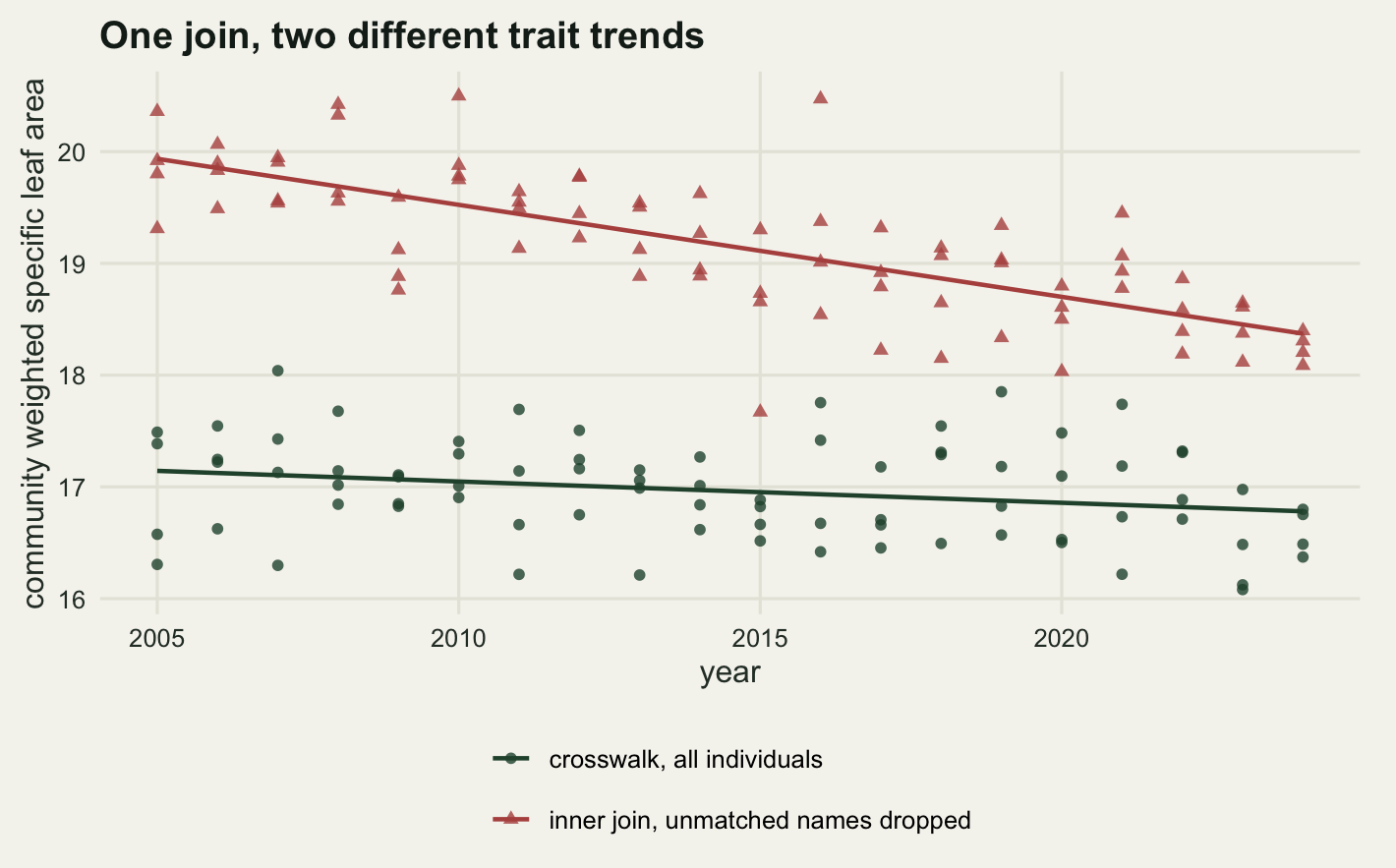
The backbone version is an analytical choice, and it is not recorded anywhere
Backbones are revised. The GBIF backbone is rebuilt, World Flora Online issues dated releases, national checklists get new editions. Running the same script a year apart can therefore produce different numbers with no change to the data and no change to the code. That is easy to say and rarely quantified, so here is the size of it. Version B below differs from version A by toggling the lumping decision in eight families and by leaving two genus transfers unmade; the counts, the traits and the analysis are identical.
set.seed(20260808)
multi_fam <- unique(fam[duplicated(fam) | duplicated(fam, fromLast = TRUE)])
toggle <- sample(multi_fam, 8)
nm24b <- nm24
for (f in toggle) {
  g <- which(fam == f)
  if (length(unique(nm24[g])) == 1) nm24b[g] <- tag(g) else nm24b[g] <- tag(min(g))
}
for (i in moved[1:2]) nm24b[nm24 == nm24[i]] <- tag(i)

answer_under <- function(key) {
  rr <- rich_of(key)
  cm <- aggregate(Y, by = list(species = key), FUN = sum)
  jj <- merge(cm, traits, by = "species")
  Jm <- as.matrix(jj[, ab_cols])
  cw <- as.vector(colSums(Jm * jj$sla) / colSums(Jm))
  c(accepted_names = length(unique(key)), mean_richness = mean(rr),
    richness_per_decade = unname(coef(lm(rr ~ pt$t_c))[2]) * 10,
    mean_cwm = mean(cw), cwm_per_decade = unname(coef(lm(cw ~ pt$t_c))[2]) * 10,
    abundance_kept_pct = 100 * sum(Jm) / sum(Y))
}

ver <- rbind(version_A = answer_under(nm24), version_B = answer_under(nm24b))
print(round(ver, 4))
accepted_names mean_richness richness_per_decade mean_cwm
version_A 69 44.2000 -3.2556 19.1535
version_B 62 40.5375 -3.3327 18.7630
cwm_per_decade abundance_kept_pct
version_A -0.8234 82.1440
version_B -0.7455 87.8741abs_gap <- function(col) unname(abs(ver[1, col] - ver[2, col]))
pct_gap <- function(col) 100 * abs_gap(col) / abs(ver[1, col])
print(c(taxa_reassigned = sum(membership(nm24) != membership(nm24b))))taxa_reassigned
19 print(round(c(richness_gap = abs_gap("mean_richness"),
richness_gap_pct = pct_gap("mean_richness"),
richness_trend_gap = abs_gap("richness_per_decade"),
richness_trend_gap_pct = pct_gap("richness_per_decade"),
cwm_trend_gap = abs_gap("cwm_per_decade"),
cwm_trend_gap_pct = pct_gap("cwm_per_decade")), 4)) richness_gap richness_gap_pct richness_trend_gap
3.6625 8.2862 0.0771
richness_trend_gap_pct cwm_trend_gap cwm_trend_gap_pct
2.3672 0.0779 9.4641 Eight toggled families and two unmade transfers reassign 19 of 80 recorded names, and the result goes against what I expected to find. The level moves a good deal: mean richness differs by 3.6625 taxa per visit, or 8.286 per cent, which is more than a rounding difference in any table of site richness. The same two versions move the richness trend by 0.0771 taxa per decade, which is 2.367 per cent of itself. The trait trend moves proportionally more, 0.0779 units per decade or 9.464 per cent, and that comparison is not a clean test of the version choice: the trait table stays keyed on the 2005 names while the community matrix is re-keyed, so the share of individuals surviving the join moves from 82.144 to 87.874 per cent as well. Whether that changes a conclusion depends on which of those numbers a conclusion rests on.
None of that is an all-clear. The damage in the earlier sections came from the same map being applied inconsistently: to one half of a series and not the other, or to a community matrix and not to a trait table. The version is still worth recording, for the same reason a seed is worth recording, because a reader who reruns the script next year gets 40.538 taxa a visit instead of 44.2 has no way to tell whether the data changed or the backbone did. Garnett and Christidis (2017) argued for a governed, versioned list precisely because the alternative is a moving reference that nobody cites.
Three ways to handle an era break, and what each one saves
Now put the pieces together in the situation that started the post. The first ten years were recorded under the 2005 concepts; the last ten under the 2024 concepts. The generating truth is known throughout, because the underlying taxa never changed, only the names applied to them, and truth here means richness counted in the 2024 concepts across the whole period.
Three treatments. Harmonise everything to the newest backbone, which for the old half means pushing each 2005 name onto one 2024 name, because a record written under a coarse concept cannot be split after the fact. Aggregate everything to the coarsest common concept. Or analyse the two eras separately and compare the conclusions.
era1 <- pt$year <= 2014
rep_24 <- vapply(split(seq_len(n_tx), nm05),
                 function(g) nm24[g[which.min(g)]], character(1))
key_truth <- matrix(nm24, n_tx, nrow(pt))
key_harm <- key_truth
key_harm[, era1] <- rep_24[nm05]
key_coarse <- matrix(cc, n_tx, nrow(pt))
key_era <- key_truth
key_era[, era1] <- nm05

rich_matrix <- function(K)
  vapply(seq_len(ncol(Y)), function(j) length(unique(K[Y[, j] > 0, j])), integer(1))
r_truth <- rich_matrix(key_truth)
r_harm <- rich_matrix(key_harm)
r_coarse <- rich_matrix(key_coarse)
r_era <- rich_matrix(key_era)

slope_sub <- function(v, keep) {
  m <- lm(v[keep] ~ pt$t_c[keep])
  c(per_decade = unname(coef(m)[2]) * 10, lo = confint(m)[2, 1] * 10,
    hi = confint(m)[2, 2] * 10)
}
all_rows <- rep(TRUE, nrow(pt))
treat <- rbind(truth = slope_sub(r_truth, all_rows),
               harmonised_to_2024 = slope_sub(r_harm, all_rows),
               common_concept = slope_sub(r_coarse, all_rows),
               era_1_alone = slope_sub(r_era, era1),
               era_2_alone = slope_sub(r_era, !era1))
print(round(treat, 4))
per_decade lo hi
truth -3.2556 -4.7409 -1.7703
harmonised_to_2024 2.4699 1.0858 3.8541
common_concept -2.1335 -3.2152 -1.0517
era_1_alone -0.6212 -3.6897 2.4472
era_2_alone -2.8182 -7.1485 1.5122print(round(c(truth_era1 = mean(r_truth[era1]), truth_era2 = mean(r_truth[!era1]),
harm_era1 = mean(r_harm[era1]), harm_era2 = mean(r_harm[!era1]),
coarse_era1 = mean(r_coarse[era1]),
coarse_era2 = mean(r_coarse[!era1])), 3)) truth_era1 truth_era2 harm_era1 harm_era2 coarse_era1 coarse_era2
45.900 42.500 38.700 42.500 38.700 36.425 print(round(c(true_step = mean(r_truth[!era1]) - mean(r_truth[era1]),
harmonised_step = mean(r_harm[!era1]) - mean(r_harm[era1]),
harmonised_era1_deficit = mean(r_truth[era1]) - mean(r_harm[era1]),
harmonised_era2_deficit = mean(r_truth[!era1]) - mean(r_harm[!era1])),
4)) true_step harmonised_step harmonised_era1_deficit
-3.4 3.8 7.2
harmonised_era2_deficit
0.0 print(c(harmonised_equals_coarse_in_era_1 = all(r_harm[era1] == r_coarse[era1]),
harmonised_equals_truth_in_era_2 = all(r_harm[!era1] == r_truth[!era1])))harmonised_equals_coarse_in_era_1 harmonised_equals_truth_in_era_2
TRUE TRUE The truth is a decline of 3.2556 taxa per decade, interval -4.7409 to -1.7703, which a twenty-year scheme detects. Harmonising everything to the newest backbone returns 2.4699 taxa per decade, interval 1.0858 to 3.8541. That is the true decline pulled upward, and the mechanism is visible in the era means: the harmonised series understates era-one richness by 7.2 taxa a visit while its era-two deficit is 0. Old records cannot be split into new concepts, new records need no splitting, so the deficit falls entirely on the first half of the series and the artefact is a step. The step is 3.8 taxa where the true step was -3.4.
The last two lines of the chunk say something sharper than the numbers do. The harmonised series is identical to the coarsest-common-concept series at every visit in era one and identical to the truth at every visit in era two, so harmonising to the newest backbone is not a third treatment at all: it is the coarse treatment on the old half and the fine treatment on the new half, stitched together at the era boundary. Both halves are defensible; the seam between them is not.
The coarsest common concept returns -2.1335 taxa per decade, interval -3.2152 to -1.0517. Correct sign, correct order of magnitude, attenuated by 34.469 per cent. Its era means are 38.7 and 36.425, so the level is depressed in both halves by the same mechanism and the comparison between them survives.
Analysing the eras separately gives -0.6212 taxa per decade in the first, interval -3.6897 to 2.4472, and -2.8182 in the second, interval -7.1485 to 1.5122. Both intervals contain zero. Ten annual visits to four plots cannot resolve a decline of 3.2556 taxa a decade, so the honest conclusion from this treatment is that neither era shows detectable change. That is not a wrong answer; it is a weaker one, bought by refusing to combine.
lab_tr <- c("truth (2024 concepts throughout)", "harmonised to the 2024 backbone",
            "coarsest common concept")
tr_dat <- data.frame(
  year = rep(pt$year, 3),
  richness = c(r_truth, r_harm, r_coarse),
  series = factor(rep(lab_tr, each = nrow(pt)), levels = lab_tr))

ggplot(tr_dat, aes(year, richness, colour = series, shape = series)) +
  geom_vline(xintercept = 2014.5, colour = te_pal$line, linetype = "22",
             linewidth = 0.8) +
  geom_point(size = 1.7, alpha = 0.75) +
  geom_smooth(method = "lm", formula = y ~ x, se = FALSE, linewidth = 0.8) +
  scale_colour_manual(values = c(te_pal$forest, te_pal$clay, te_pal$gold),
                      name = NULL) +
  scale_shape_manual(values = c(16, 17, 15), name = NULL) +
  guides(colour = guide_legend(nrow = 2), shape = guide_legend(nrow = 2)) +
  labs(x = "year", y = "taxa recorded per visit",
       title = "Three treatments of one era break") +
  theme_te() +
  theme(plot.margin = margin(8, 14, 4, 8))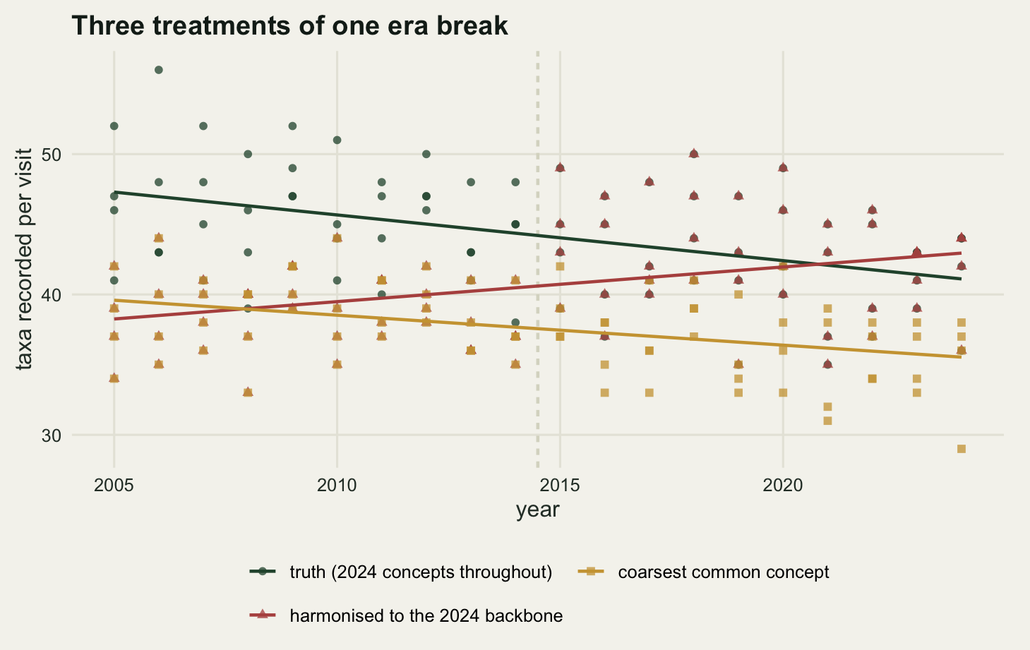
Reading the three treatments against each other: harmonising to the newest backbone does not recover the true slope, and it is the one the standard advice recommends. It goes wrong because the map from old records to new names is not invertible and the analysis pretended it was. The coarse concept kept the sign at the cost of 34.469 per cent of the slope and 6.638 taxa of the level. The separate analysis kept everything except the ability to say anything.
None of the three is free and there is no fourth option that keeps all of it, so what the report can do is name the choice. A methods sentence of the form “records were harmonised to the national checklist version 2024.1; segregate pairs lumped by that revision were also lumped in the pre-2015 data, so trends for those taxa are aggregate trends” costs one line and tells a reader which of the three prices was paid.
What to take away
Harmonisation is not data cleaning. Cleaning removes errors: two spellings of one plant were never two plants, and collapsing them restores something true. Harmonisation applies a many-to-one map to records that were correct as written, and the entities it removes were real distinctions that somebody in the field could see.
The measurements put sizes on that. Two segregates trending at 5.975 and -4.655 per cent a year became one aggregate at 0.574 per cent with a p value of 0.1718. The sweep found a window of real declines, -0.02 to -0.05 on the log scale, that the segregate’s own series detects with near certainty and the aggregate essentially never does: 4 times steeper is what the aggregate needs. Aggregating a whole flora to the coarsest common concept cost 15.017 per cent of the richness and 34.469 per cent of the richness trend, the second larger than the first. An inner join between a trait table on old names and a matrix on new ones dropped 17.856 per cent of the individuals in silence.
Two results went against expectation, and both stay in. The backbone version, which I expected to be a substantial source of variation, shifted mean richness by 8.286 per cent but the richness trend by only 2.367 per cent: a uniform relabelling is a level effect, and slopes do not see it. And the trait-join example did not reverse its sign on the first draw, as I had assumed it would. It did something quieter, turning a slope of -0.1904 units per decade into one of -0.8234.
The treatment comparison also produced something I had not planned to find. Harmonising the old half of a series onto the new backbone is arithmetically the same as applying the coarsest common concept to that half alone, the two richness series agreeing at every visit in era one, so the recommended route is not a distinct choice between the other two. It is both of them at once, one per era, and the seam returned 2.4699 taxa per decade against a truth of -3.2556.
The honest limit is that none of these costs is visible from inside the harmonised dataset. Every diagnosis above used something the analyst does not have: the generating trends of the two segregates, the true concept identity of every record, the trait value of every dropped taxon. Given only the harmonised table, the flat aggregate trend, the depressed richness and the joined trait trend all look like ordinary results, and the sweep says the blind window is wide. There is no residual to check and no warning to catch. What is available is the crosswalk itself: it is a table, it can be read before it is applied, and counting how much abundance sits on its many-to-one rows takes one line and tells you which of the numbers above you are about to pay. Nothing downstream will tell you afterwards.
References
Isaac NJB, Mallet J, Mace GM 2004 Trends in Ecology and Evolution 19(9):464-469 (10.1016/j.tree.2004.06.004)
Garnett ST, Christidis L 2017 Nature 546(7656):25-27 (10.1038/546025a)
Grenie M, Berti E, Carvajal-Quintero J, Dadlow GML, Sagouis A, Winter M 2023 Methods in Ecology and Evolution 14(1):12-25 (10.1111/2041-210X.13802)
Meyer C, Weigelt P, Kreft H 2016 Ecology Letters 19(8):992-1006 (10.1111/ele.12624)
Chamberlain SA, Szocs E 2013 F1000Research 2:191 (10.12688/f1000research.2-191.v2)
Jin Y, Qian H 2019 Ecography 42(8):1353-1359 (10.1111/ecog.04434)
Kattge J, et al 2020 Global Change Biology 26(1):119-188 (10.1111/gcb.14904)
Legendre P, Legendre L 2012 Numerical Ecology, third edition (ISBN 978-0-444-53868-0)