Records on grid lines and floating point in R

One-decimal records sit on the lines of a 0.1 degree atlas grid. Count how floor(), terra and sf place them, and assign cells in R with integer arithmetic.

A plant atlas maps records in cells of 0.1 degree, from 20 to 30 degrees east and from 44 to 48 degrees north: one hundred columns and forty rows. The records come from herbarium sheets and an online occurrence export, and they carry coordinates to one decimal place, 23.4 east, 46.7 north. The column of a record is worked out the way a textbook would put it: subtract the western edge of the atlas, divide by the cell size, round down. floor((lon - 20) / 0.1). The map that comes out has empty columns in a regular pattern, each one beside a column with twice the records.

Every one-decimal longitude on this atlas lies exactly on a cell edge, so every record depends on how the arithmetic settles a tie that exists in the decimal number but not in the binary number R stores. This post counts what three common routes do with such records: the formula above, cellFromXY() from terra, and a spatial join with sf. It then shows the fix, which is to decide first which cell owns a point on a line and then to do the cell arithmetic in whole numbers.

Floating point has come up on this site before, in a narrower form. Pinning package versions with renv shows two routes to the same sum disagreeing in the last bits and says this matters “at exactly one place: an equality test”. Checking an analysis script finds that the usual worry about summation order is misplaced for its totals. A cell index is an equality test in disguise, and it is where the last bits decide something. Snapped coordinates and a clustering verdict grids continuous coordinates into cells of whole units, where no record sits on a line, and Rounded and coarsened measurements is about what rounding does to statistics, not to which cell a value lands in. Mapping species richness in R with sf joins records to a grid with st_join(); its records have continuous coordinates, so the question of a record on a cell edge does not arise there.

The short answer. Decimal fractions such as 0.1 and 20.2 are stored in binary as the nearest representable number, which is a little above or a little below the value you typed. On a grid line that difference decides the cell. Choose an edge rule before you grid anything (here: a cell owns its western and southern edges), turn the coordinates into whole numbers of the smallest unit you trust with round(), and compute the cell index with integer division. Hand terra or sf the cell centre, not the raw record.

The records below are synthetic and the seed is in the code. The misassignment shares are counts over every grid-line value, not Monte Carlo estimates: the random records only decide how often each value occurs.

library(ggplot2)
library(terra)
library(sf)

te_paper  <- "#f5f4ee"
te_ink    <- "#16241d"
te_body   <- "#2c3a31"
te_forest <- "#275139"
te_rust   <- "#b5534e"
te_gold   <- "#c9b458"
te_line   <- "#dad9ca"

theme_datasheet <- function() {
  theme_minimal(base_size = 12) +
    theme(plot.background  = element_rect(fill = te_paper, colour = NA),
          panel.background = element_rect(fill = te_paper, colour = NA),
          panel.grid.major = element_line(colour = te_line, linewidth = 0.3),
          panel.grid.minor = element_blank(),
          text             = element_text(colour = te_body),
          axis.text        = element_text(colour = te_body),
          strip.text       = element_text(colour = te_ink, face = "bold"),
          legend.position  = "top")
}

versions <- c(R = paste(R.version$major, R.version$minor, sep = "."),
              terra = packageDescription("terra")$Version,
              sf = packageDescription("sf")$Version)
terra_year <- sub("^NA$", "n.d.", format(utils::packageDate("terra"), "%Y"))
versions

       R    terra       sf 
 "4.5.3" "1.9-34"  "1.1-1" 

A tenth is not stored as a tenth

Start away from maps. A sediment core is cut into slices every 10 cm and the depths are generated with seq(); four depths that went to the lab are typed in by hand.

depth <- seq(0, 2, by = 0.1)                # slice depths, metres
typed <- c(0.3, 0.6, 0.7, 1.2)              # depths typed from the lab sheet
stopifnot(identical(depth, 0 + (0:20) * 0.1))   # seq() builds from + i * by
found       <- sum(depth %in% typed)
same_typed  <- sum(depth == round(depth, 1))
found_round <- sum(round(depth, 1) %in% typed)
c(found = found, seq_equal_to_typed = same_typed, of = length(depth),
  found_after_round = found_round)

             found seq_equal_to_typed                 of  found_after_round 
                 0                 14                 21                  4 

sprintf("%.20f", c(seq_value = depth[4], typed_value = 0.3))

[1] "0.30000000000000004441" "0.29999999999999998890"

gap_03 <- depth[4] - 0.3
stopifnot(gap_03 == 2^-54)                   # one binary step at this size

%in% looks for exact matches and finds 0 of the 4 depths. seq() builds each value as the start plus i times the step, and 3 * 0.1 is not the same binary number as the 0.3 the parser makes from the text “0.3”; the two differ by \(5.55 \times 10^{-17}\), which is 2 to the power -54, one step of the binary number line at this size. Of the 21 depths, 14 equal the value you would get by typing them and 7 do not. round(depth, 1) maps each one back to the nearest typed value, and then all 4 are found. This is the problem question 7.31 of the R FAQ answers (Hornik and R Core Team 2023; its own examples are sqrt(2) * sqrt(2) == 2 and .3 + .6 == .9), and Goldberg (1991) explains the arithmetic behind it. So far nothing is new: compare with a tolerance, or round first.

One formula, one hundred longitudes

The atlas is the same problem at every record. Its edge rule is written down before any arithmetic: a cell includes its western and southern edges, so the column of longitude 23.4 is the cell from 23.4 to 23.5, column 34 counted from 0. In whole tenths of a degree that rule is exact: 23.4 is 234 tenths, and 234 minus 200 is 34.

The chunk below takes all 100 one-decimal longitudes of the atlas, from 20.0 to 29.9, parsed from text as they would be read from a file, and computes the column three ways: dividing by 0.1, multiplying by 10, and in whole tenths.

x0 <- 20; y0 <- 44; cell <- 0.1                          # atlas origin and cell size, degrees
lon_values <- as.numeric(sprintf("%.1f", 200:299 / 10))    # 20.0, 20.1, ..., 29.9
tenths     <- round(lon_values * 10)                       # whole tenths: exact
cols <- data.frame(lon = lon_values,
                   intended = tenths - 200,                # the edge rule, in integers
                   divide   = floor((lon_values - x0) / cell),
                   multiply = floor((lon_values - x0) * 10))
wrong_col <- colSums(cols[, c("divide", "multiply")] != cols$intended)
stopifnot(all(cols$divide[cols$multiply != cols$intended] != cols$intended[cols$multiply != cols$intended]))
wrong_col

  divide multiply 
      40       33 

table(divide_minus_intended = cols$divide - cols$intended)

divide_minus_intended
-1  0 
40 60 

wrong_lon <- cols$lon[cols$divide != cols$intended]
wrong_per_degree <- table(floor(wrong_lon))
wrong_tenths <- sort(unique(round(wrong_lon * 10) %% 10))
c(values_per_degree = unique(as.vector(wrong_per_degree)))

values_per_degree 
                4 

sprintf("%.20f", c(lon = 20.2, minus_origin = 20.2 - x0, divided = (20.2 - x0) / cell))

[1] "20.19999999999999928946" "0.19999999999999928946" 
[3] "1.99999999999999289457" 

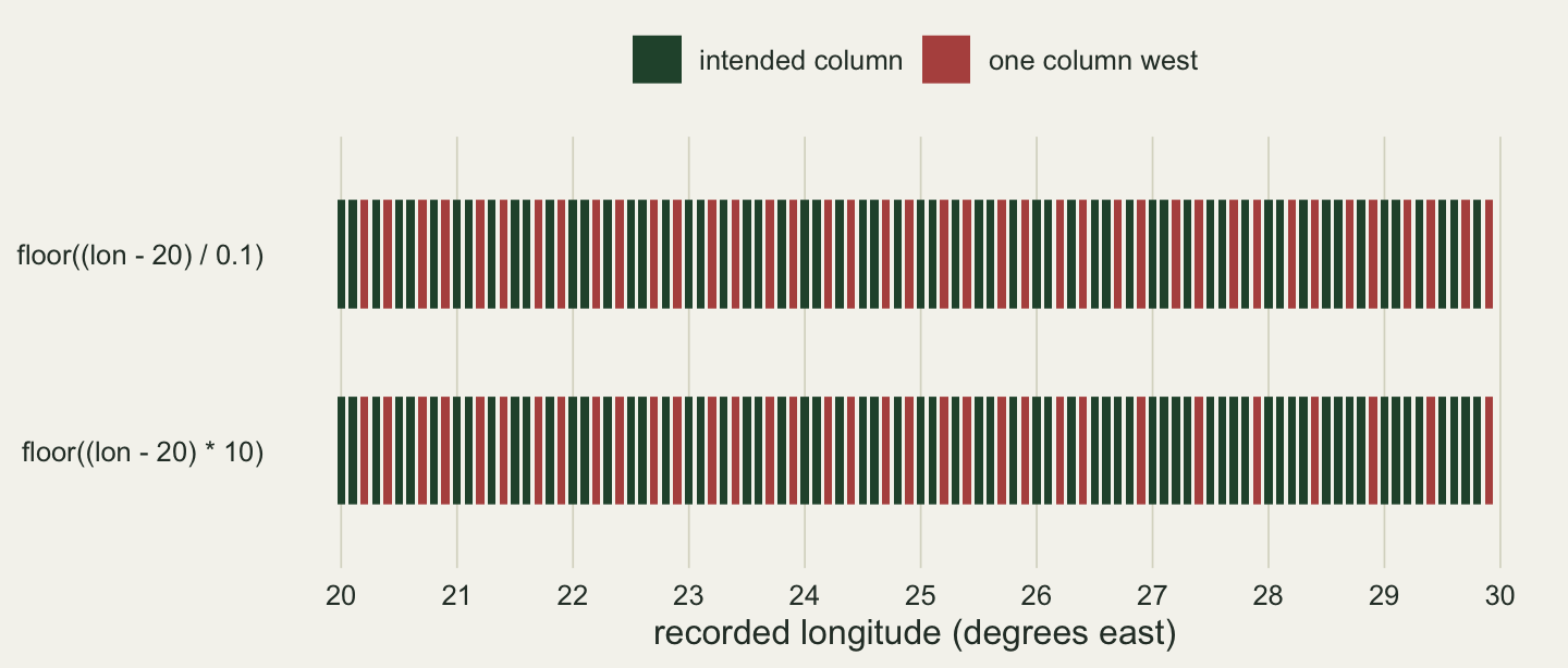
floor((lon - 20) / 0.1) puts 40 of the 100 longitudes in the wrong column, and every one of them one column to the west. In every degree they are the same 4 values, those ending in .2, .4, .7, .9. The last line shows why for 20.2. The stored number is slightly below 20.2; subtracting 20 is exact and leaves the small error standing next to a small number, so the difference is 0.19999999999999929: the tiny error of 20.2 now sits beside a number a hundred times smaller, and relative to that number it is a hundred times larger. Dividing by the stored 0.1, which is slightly above one tenth, lowers it again, and floor() of 1.99999999999999 is 1. Multiplying by 10 instead gets 33 wrong, all of them among the 40 (the stopifnot() line checks this). Neither route is careless; both ask floor() to settle a tie that only exists in decimal.

Figure 1: All 100 one-decimal longitudes of the atlas, each on a cell edge, and the column two formulas give them. Each bar is one recorded value: rust bars land one column west of the column the edge rule assigns, green bars land where the rule puts them. The integer rule is correct by construction, so it is not drawn.

How many values go wrong depends on the origin, the cell size and the number of decimals. The next chunk repeats the count for other grids. Each row is an exact enumeration of every recorded value in a span of ten degrees (four for the latitude row); there is no sampling in it.

count_wrong <- function(origin, cell_units, dec, span = 10) {
  # cell_units: the cell size in units of the last recorded decimal
  k <- round(origin * 10^dec) + 0:(span * 10^dec - 1)          # every value, in integers
  v <- as.numeric(sprintf(paste0("%.", dec, "f"), k / 10^dec))  # as read from text
  cell_size <- cell_units / 10^dec
  intended  <- (k - round(origin * 10^dec)) %/% cell_units
  on_line   <- (k - round(origin * 10^dec)) %% cell_units == 0
  divide    <- floor((v - origin) / cell_size)
  c(values = length(v), on_a_line = sum(on_line), wrong = sum(divide != intended),
    wrong_off_a_line = sum(divide != intended & !on_line))
}
grids <- rbind(
  "lon from 20, 0.1 cells, 1 decimal"   = count_wrong(20, 1, 1),
  "lon from 16, 0.1 cells, 1 decimal"   = count_wrong(16, 1, 1),
  "lat from 44, 0.1 cells, 1 decimal"   = count_wrong(44, 1, 1, span = 4),
  "lon from 20, 0.5 cells, 1 decimal"   = count_wrong(20, 5, 1),
  "lon from 15.9, 0.5 cells, 1 decimal" = count_wrong(15.9, 5, 1),
  "lon from 20, 0.1 cells, 2 decimals"  = count_wrong(20, 10, 2),
  "lon from 20, 0.05 cells, 2 decimals" = count_wrong(20, 5, 2),
  "lon from 20, 0.25 cells, 2 decimals" = count_wrong(20, 25, 2),
  "lon from 20, 0.01 cells, 2 decimals" = count_wrong(20, 1, 2))
grids

                                    values on_a_line wrong wrong_off_a_line
lon from 20, 0.1 cells, 1 decimal      100       100    40                0
lon from 16, 0.1 cells, 1 decimal      100       100    40                0
lat from 44, 0.1 cells, 1 decimal       40        40    16                0
lon from 20, 0.5 cells, 1 decimal      100        20     0                0
lon from 15.9, 0.5 cells, 1 decimal    100        20    19                0
lon from 20, 0.1 cells, 2 decimals    1000       100    40                0
lon from 20, 0.05 cells, 2 decimals   1000       200    80                0
lon from 20, 0.25 cells, 2 decimals   1000        40     0                0
lon from 20, 0.01 cells, 2 decimals   1000      1000   423                0

stopifnot(all(grids[, "wrong_off_a_line"] == 0))
whole_origins <- sapply(-179:179, function(o) count_wrong(o, 5, 1)[["wrong"]] + count_wrong(o, 25, 2)[["wrong"]])
stopifnot(all(whole_origins == 0))    # 0.5 and 0.25 cells from every whole-degree origin

Two things hold in every row. Only values on a line are ever misplaced (the last column is zero throughout), and the share at risk is the share on a line: all of them for one-decimal records on a 0.1 grid, one in ten for two-decimal records on the same grid. Among the values on a line, the share that goes wrong is not a constant. It is 40 of 100 for the atlas longitudes, 16 of 40 for its latitudes and 423 of 1000 for a 0.01 degree grid, and it is zero for 0.5 and 0.25 degree cells that start on a whole degree, because a half and a quarter are exact in binary and so is every line of such a grid (the second stopifnot() checks every whole-degree origin from 179 west to 179 east). The origin has to be exact too: the same 0.5 degree cells starting at 15.9 misplace 19 of 20 values on a line. The count also depends on the magnitude of the coordinates, so check it on your own extent rather than borrowing these.

What the stripes do to an atlas map

The atlas gets 20000 synthetic records, one decimal in each coordinate, with every value in the atlas equally likely. Rows are assigned the same two ways as columns.

set.seed(2210)
n_rec <- 20000
lon_k <- sample(200:299, n_rec, replace = TRUE)            # tenths of a degree
lat_k <- sample(440:479, n_rec, replace = TRUE)
records <- data.frame(lon = as.numeric(sprintf("%.1f", lon_k / 10)),
                      lat = as.numeric(sprintf("%.1f", lat_k / 10)))
col_rule  <- round(records$lon * 10) - 200                 # edge rule, integers
row_rule  <- round(records$lat * 10) - 440
col_floor <- floor((records$lon - x0) / cell)
row_floor <- floor((records$lat - y0) / cell)
per_cell <- function(col, row) tabulate(row * 100 + col + 1, nbins = 4000)
n_rule  <- per_cell(col_rule, row_rule)
n_floor <- per_cell(col_floor, row_floor)
lat_values <- as.numeric(sprintf("%.1f", 440:479 / 10))
wrong_lat  <- sum(floor((lat_values - y0) / cell) != 0:39)
share_expected <- 1 - (1 - wrong_col[["divide"]] / 100) * (1 - wrong_lat / 40)
share_moved    <- mean(col_floor != col_rule | row_floor != row_rule)
c(empty_cells_rule = sum(n_rule == 0), empty_cells_floor = sum(n_floor == 0),
  max_per_cell_rule = max(n_rule), max_per_cell_floor = max(n_floor),
  share_expected = share_expected, share_moved = share_moved,
  empty_expected_by_chance = 4000 * (1 - 1 / 4000)^n_rec)

        empty_cells_rule        empty_cells_floor        max_per_cell_rule 
                21.00000               2085.00000                 15.00000 
      max_per_cell_floor           share_expected              share_moved 
                36.00000                  0.64000                  0.64105 
empty_expected_by_chance 
                26.93495 

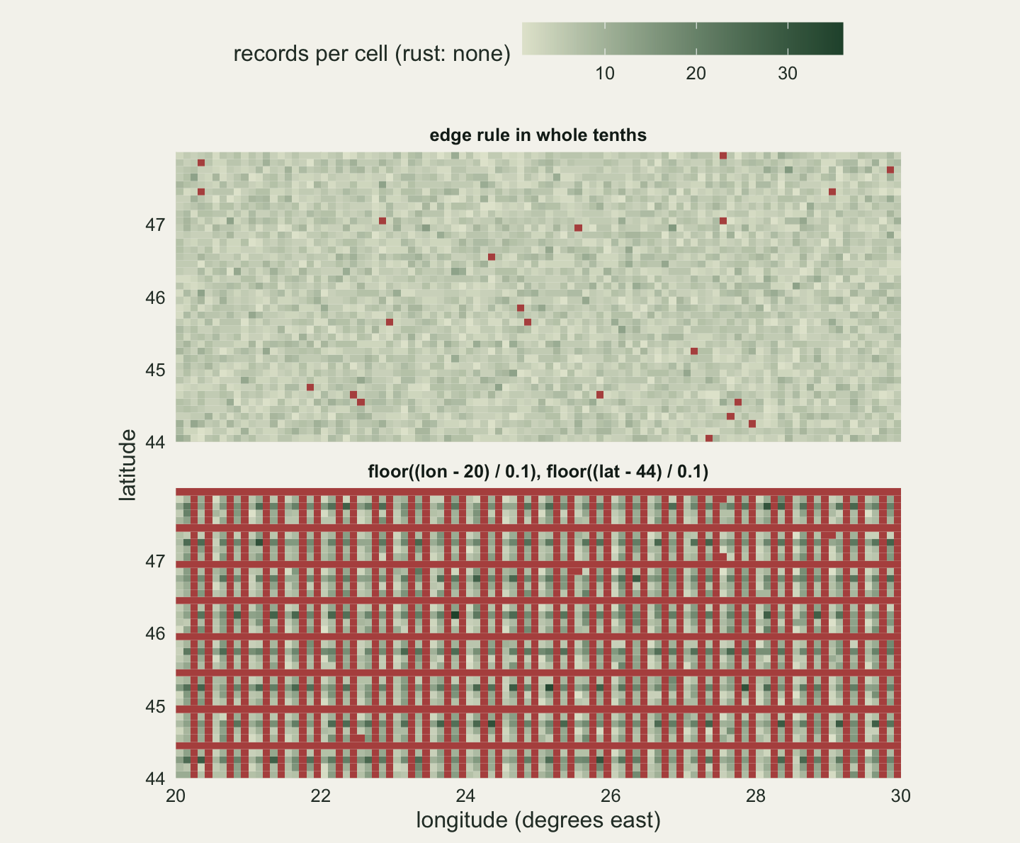
A record keeps its cell only if both its column and its row come out right. With every value equally likely, that has probability (1 - 40/100) times (1 - 16/40), so the expected share of records in the wrong cell is 0.64: arithmetic, not a simulation result. Of the 20000 drawn records a share of 0.6411 is in the wrong cell, which differs from 0.64 only because the draw does not hit every value equally often. Under the edge rule 21 of the 4000 cells have no record, in line with the 26.9 that chance alone leaves empty on average at five records per cell. Under floor() 2085 cells are empty and the fullest cell holds 36 records against 15. The empty cells are not scattered. A misplaced value moves into the neighbouring column or row; where nothing moves in to replace it, its own is left empty and the neighbour holds twice the records. So the map shows stripes, and a richness or occupancy map built on it has gaps that look like a survey pattern.

Figure 2: Records per 0.1 degree cell for the same 20000 synthetic one-decimal records, gridded with the edge rule in whole tenths (top) and with floor((coordinate - origin) / 0.1) (bottom). Empty cells are rust.

terra: its own rule, and the same arithmetic

cellFromXY() in terra (Hijmans 2026) has an edge rule of its own. Its help page (terra 1.9-50, the CRAN version when this was written) says that a point on the edge of two or four cells goes to the cell on the right, the cell below, or on a corner the cell below and to the right, and a comment in the C++ source adds that points on the right-hand and bottom edges of the raster are kept inside. The first lines of the chunk check all three cases and both edges on a small raster of 0.5 degree cells, where every coordinate is exact in binary. So terra’s column rule is the atlas rule, and its row rule is the opposite one: a record on 46.7 north belongs to the cell from 46.6 to 46.7. The chunk compares what cellFromXY() returns for every grid-line longitude and latitude with terra’s own stated rule.

r05 <- rast(xmin = 20, xmax = 22, ymin = 44, ymax = 46, resolution = 0.5)
rc <- rowColFromCell(r05, cellFromXY(r05, rbind(c(21, 45.25), c(20.75, 45), c(20.75, 44), c(22, 45.25), c(21, 45))))
stopifnot(rc[1, 2] == 3, rc[2, 1] == 3, rc[3, 1] == 4, rc[4, 2] == 4, rc[5, ] == 3)   # right, below, corner; outer edges inside
atlas_r <- rast(xmin = 20, xmax = 30, ymin = 44, ymax = 48, resolution = 0.1)
col_terra <- colFromCell(atlas_r, cellFromXY(atlas_r, cbind(lon_values, 46.05))) - 1   # 0 = west
row_terra <- rowFromCell(atlas_r, cellFromXY(atlas_r, cbind(25.05, lat_values)))
row_below <- 40 - (0:39) + 1                  # row, counted from the top, just below the line
row_below[lat_values == 44] <- 40             # the bottom edge goes up into the raster
terra_col_off <- sum(col_terra != cols$intended)
terra_row_off <- sum(row_terra != row_below)
terra_same_as_multiply <- identical(as.numeric(col_terra), as.numeric(cols$multiply))
c(columns_off_rule = terra_col_off, of = length(lon_values),
  rows_off_rule = terra_row_off, of = length(lat_values),
  columns_as_floor_times_10 = terra_same_as_multiply)

         columns_off_rule                        of             rows_off_rule 
                       33                       100                        16 
                       of columns_as_floor_times_10 
                       40                         1 

cell_terra <- cellFromXY(atlas_r, as.matrix(records))
n_terra    <- tabulate(cell_terra, nbins = ncell(atlas_r))
top_row_records <- sum(n_terra[1:100])        # cells 1 to 100: the row from 47.9 to 48
c(empty_cells_terra = sum(n_terra == 0), records_in_top_row = top_row_records)

 empty_cells_terra records_in_top_row 
              1862                  0 

With terra 1.9-34 on this page, 33 of the 100 grid-line longitudes land one column west of the column terra’s rule gives, and 16 of the 40 latitudes land in the row above the line instead of below it. Its columns are exactly those of floor((lon - 20) * 10) from the chunk before, because it computes the column the same way: subtract the western edge, multiply by the number of columns per degree, round down. On the 20000 records, 1862 of the 4000 cells of the raster are empty. Two causes are mixed in that count: the stripes from misplaced values, and the difference between terra’s row rule and the atlas rule. Under terra’s rule the records on 47.9 north belong to the row below, no record reaches the top row from 47.9 to 48, and all 100 of its cells are empty. None of this is a fault in terra. A point on a shared edge has no correct cell until somebody chooses a rule; terra chose one and writes it down, and floating point decides whether a given record meets it.

sf: a record on a corner belongs to four cells

A spatial join asks a different question. st_join() pairs each point with every cell polygon it intersects (its default predicate is st_intersects), and a point on a shared edge intersects both cells. The grid below is the same atlas made with st_make_grid() from sf (Pebesma 2018). Spherical geometry is switched off so that sf treats longitude and latitude as plain x and y, the way the atlas is drawn.

stopifnot(identical(formals(sf:::st_join.sf)$join, quote(st_intersects)))
invisible(suppressMessages(sf_use_s2(FALSE)))
atlas_bbox <- st_as_sfc(st_bbox(c(xmin = 20, ymin = 44, xmax = 30, ymax = 48), crs = 4326))
atlas_sf <- st_sf(cell = 1:4000, geometry = st_make_grid(atlas_bbox, cellsize = 0.1))
rec_sf   <- st_as_sf(records, coords = c("lon", "lat"), crs = 4326, remove = FALSE)
cells_hit <- lengths(suppressMessages(st_intersects(rec_sf, atlas_sf)))
joined    <- suppressMessages(st_join(rec_sf, atlas_sf))
within_n  <- lengths(suppressMessages(st_within(rec_sf, atlas_sf)))
c(records = nrow(rec_sf), joined_rows = nrow(joined), sum_cells_hit = sum(cells_hit))

      records   joined_rows sum_cells_hit 
        20000         76971         76971 

table(cells_per_record = cells_hit)

cells_per_record
    1     2     4 
   29  1471 18500 

table(cells_within = within_n)

cells_within
    0 
20000 

line_x <- sort(unique(st_coordinates(atlas_sf)[, "X"]))   # the lines sf computes, axis by axis
line_y <- sort(unique(st_coordinates(atlas_sf)[, "Y"]))
inner_x <- line_x[-c(1, length(line_x))]; inner_y <- line_y[-c(1, length(line_y))]
touch_x <- 1 + records$lon %in% inner_x
touch_y <- 1 + records$lat %in% inner_y
stopifnot(all(cells_hit == touch_x * touch_y), sum(cells_hit) == nrow(joined),
          all(records$lat %in% line_y), all(within_n == 0))   # all on a latitude line; none within
off_lines <- c(line_x[!(line_x %in% c(lon_values, 30))], line_y[!(line_y %in% c(lat_values, 48))])
off_lines                                     # grid lines that are not a typed value

[1] 28.2 28.7 29.2 29.7

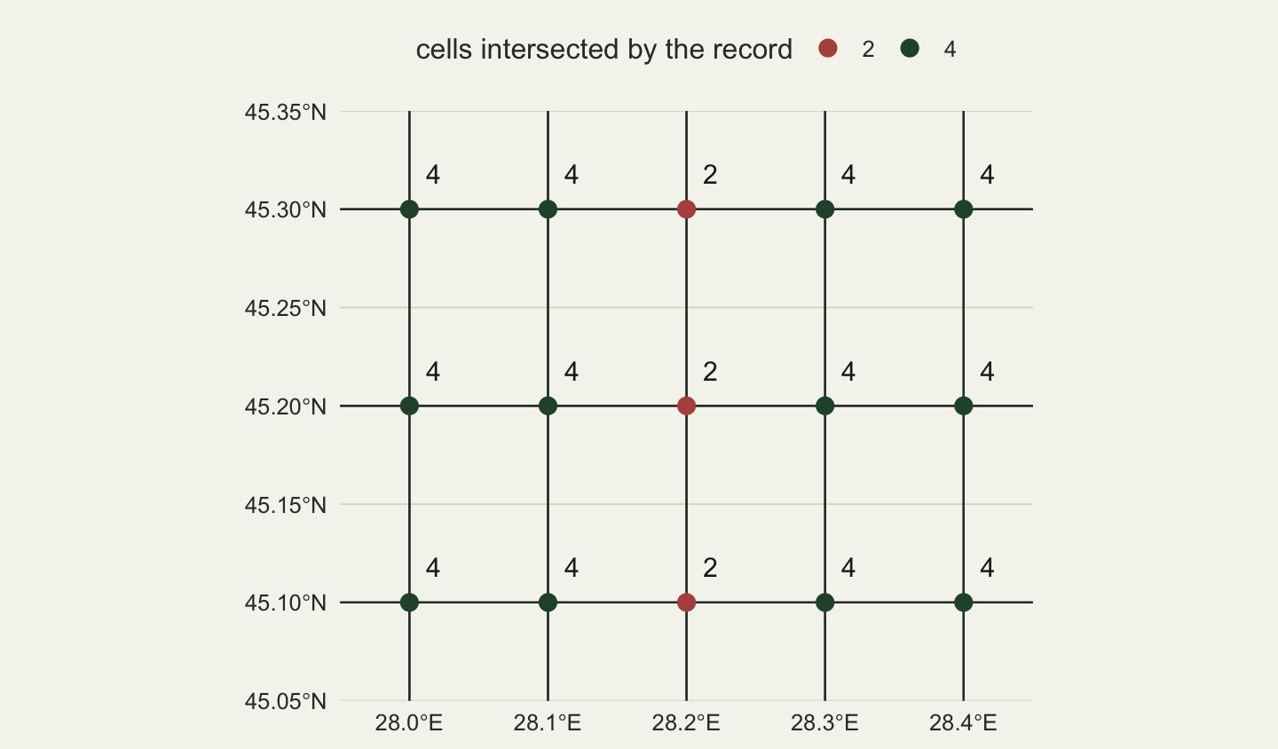
The 20000 records become 76971 rows after the join. 92.5 per cent of the records intersect four cells, 7.4 per cent two and 0.1 per cent one (sf 1.1-1). The stopifnot() line checks where each extra row comes from: the number of cells a record touches is the number of cells across its longitude line times the number across its latitude line, which is 2 by 2 on an inner corner, 2 by 1 on the outer edge of the atlas or on one of the lines described next, and 1 by 1 where two such single-sided lines meet (the south-west corner, or one of those lines at 44 north). Of the 142 grid lines that sf computes, 4, at 28.2, 28.7, 29.2, 29.7 degrees, are not the number the typed coordinate parses to (this version places line i at the origin plus i times 0.1, and for these lines that sum lands one binary step away from the typed value), so records on them touch only the cell on one side of the line. Every duplicated row is a boundary tie, and a richness count per cell built on the join counts each corner record in four cells. Changing the predicate to st_within does not help. None of the 20000 records lies within any cell, because every one of them is on a latitude line: in the geometry sf follows, a point on a polygon’s boundary is not within it, so a left join with join = st_within keeps every record and gives none of them a cell.

Figure 3: A small part of the sf atlas grid around 28 degrees east. Each point is a one-decimal record on a cell corner, labelled with the number of grid cells it intersects. Where the grid line sf computes is not the number the typed longitude parses to, the records on it touch two cells, not four.

The fix: choose the rule, then count in whole numbers

The fix has two parts, and the order matters. First write the edge rule down, in the methods and in the code: here a cell owns its western and southern edges. Then do the arithmetic in integers, where a tie is a tie. round() turns a coordinate into a whole number of small units without any doubt, because the stored number is within a tiny fraction of that whole number; integer division by the cell size in the same units then gives the index. Micro-degrees serve any record with up to six decimals (the chunk checks a sample of one hundred thousand six-decimal values between 20 and 30). They assume the numbers came from text or double-precision storage; if a coordinate may have passed through single precision (some databases and grid formats), round to the precision of the record itself, round(lon * 10) for tenths, instead.

cell_index <- function(coord, origin, cell_size) {
  micro <- round(coord * 1e6) - round(origin * 1e6)    # whole micro-degrees
  micro %/% round(cell_size * 1e6)
}
stopifnot(identical(cell_index(cols$lon, 20, 0.1), cols$intended),
          identical(cell_index(records$lon, 20, 0.1), col_rule),
          identical(cell_index(records$lat, 44, 0.1), row_rule))
two_dec <- as.numeric(sprintf("%.2f", 2000:2999 / 100))
stopifnot(all(cell_index(two_dec, 20, 0.05) == (0:999) %/% 5),
          all(cell_index(two_dec, 20, 0.01) == 0:999))
fix_ok <- function(origin, cell_units, dec, span = 10) {     # the rows of the grids table
  k <- round(origin * 10^dec) + 0:(span * 10^dec - 1)
  v <- as.numeric(sprintf(paste0("%.", dec, "f"), k / 10^dec))
  all(cell_index(v, origin, cell_units / 10^dec) == (k - round(origin * 10^dec)) %/% cell_units)
}
stopifnot(fix_ok(16, 1, 1), fix_ok(44, 1, 1, 4), fix_ok(20, 5, 1), fix_ok(15.9, 5, 1),
          fix_ok(20, 10, 2), fix_ok(20, 25, 2))
lon_single <- readBin(writeBin(lon_values, raw(), size = 4), "numeric", n = 100, size = 4)
stopifnot(identical(round(lon_single * 10) - 200, cols$intended))   # single precision: round to tenths
micro_k <- 20e6 - 1 + sample.int(10e6, 1e5)                       # six-decimal values, a sample
stopifnot(all(round(as.numeric(sprintf("%.6f", micro_k / 1e6)) * 1e6) == micro_k))
stopifnot(all(floor((0:10000) / 5) == (0:10000) %/% 5))      # whole metres, 5 m cells
c(one_decimal_floor_times_10_wrong = sum(floor(lon_values * 10) - 200 != cols$intended),
  two_decimal_floor_times_100_wrong = sum(floor(two_dec * 100) != 2000:2999))

 one_decimal_floor_times_10_wrong two_decimal_floor_times_100_wrong 
                                0                                 7 

centre_lon <- x0 + (col_rule + 0.5) * cell            # the cell centre, from the index
centre_lat <- y0 + (row_rule + 0.5) * cell
cell_from_centre <- cellFromXY(atlas_r, cbind(centre_lon, centre_lat))
centre_sf <- st_as_sf(data.frame(lon = centre_lon, lat = centre_lat),
                      coords = c("lon", "lat"), crs = 4326)
hits_centre <- lengths(suppressMessages(st_intersects(centre_sf, atlas_sf)))
stopifnot(all(colFromCell(atlas_r, cell_from_centre) - 1 == col_rule),
          all(40 - rowFromCell(atlas_r, cell_from_centre) == row_rule),
          all(hits_centre == 1))
c(records = n_rec, sf_rows_after_join = nrow(suppressMessages(st_join(centre_sf, atlas_sf))))

           records sf_rows_after_join 
             20000              20000 

The integer index agrees with the edge rule for every value in every enumeration above, including the 15.9 origin and the 0.05 and 0.01 degree cells on two-decimal records, and the stopifnot() lines make the page fail to build if it ever does not. Multiplying the raw longitude by a power of ten before anything else and rounding down happens to work for the one-decimal longitudes of this atlas (floor(lon * 10) misplaces 0 of the 100), but it is not a method: floor(lon * 100) on the thousand two-decimal longitudes from 20.00 to 29.99 gets 7 of them wrong. The step that makes the fix safe is round() to the unit, then integer arithmetic.

When the gridding has to happen in terra or sf, pass the cell centre computed from the integer index, not the record. A centre lies half a cell from every line, far beyond any rounding, so cellFromXY() returns the rule’s cell for all 20000 records and st_join() returns exactly one row per record. Keep the original coordinates in their own columns for everything else.

What to check in your own data

Count the records that sit on a line before you grid: with the coordinate in whole units of its last decimal, a record is on a line when that number is divisible by the cell size in the same units. If the count is zero, the question does not arise; each extra decimal place divides the share on a line by ten. The edge rule also needs an answer at the eastern and northern boundary: a record on 30.0 east gets column 100, outside the atlas. Decide whether such records are dropped or kept in the last column, and check all(col >= 0 & col < 100) before you tabulate. After a spatial join to a grid, compare the number of rows with the number of records. More rows means boundary ties; fewer non-missing cells than records, with st_within, means the same ties seen from the other side. Compute the cell index two ways, your production route and the integer rule, and count the disagreements. On a fresh extent or a new package version this takes one line and replaces any assumption about what a function does on an edge. In the methods, state the edge rule and how many records it decided. A reader cannot recover either from the map.

Honest limits

The counts in this post belong to one atlas: origin 20 and 44 degrees, 0.1 degree cells, one- and two-decimal records. Other origins, resolutions and magnitudes give other counts, as the table shows, and the only general statements are the two the table supports: only values on a line are at risk, and a cell size and origin that are both exact in binary (0.5 or 0.25 degree cells starting on a whole degree) are safe for decimal records; the same 0.5 degree cells starting at 15.9 are not.

An edge rule makes the assignment reproducible; it does not make it true. A coordinate given to one decimal place stands for a square about 0.1 degree across (Wieczorek and colleagues 2004 treat such coordinates as an uncertainty, not a point), and if it was rounded rather than truncated the plant could be on either side of the line. No rule places such a record correctly. When most records are that coarse, an atlas at the same resolution is mapping the recording precision as much as the plant, and a coarser atlas or an analysis that carries the uncertainty is the honest choice.

The terra and sf numbers are for terra 1.9-34 and sf 1.1-1 with spherical geometry switched off, and the prose above is computed from whatever versions build the page. With spherical geometry on, sf hands the geometry to the s2 library instead; that case was not measured. Whole numbers are exact in binary, so whole-metre coordinates on a grid of whole-metre cells from a whole-metre origin are placed exactly by floor(), ties included (the whole-metre check in the fix chunk), and continuous coordinates such as those in Snapped coordinates and a clustering verdict almost never lie on a line at all.

References

Goldberg D 1991 ACM Computing Surveys 23(1):5-48 (10.1145/103162.103163)

Hijmans RJ 2026 terra: Spatial Data Analysis. R package version 1.9-34, the version that built this page (https://CRAN.R-project.org/package=terra)

Hornik K, R Core Team 2023 The R FAQ, question 7.31 (https://CRAN.R-project.org/doc/FAQ/R-FAQ.html)

Pebesma E 2018 The R Journal 10(1):439-446 (10.32614/RJ-2018-009)

Wieczorek J, Guo Q, Hijmans RJ 2004 International Journal of Geographical Information Science 18(8):745-767 (10.1080/13658810412331280211)

Related tutorials

• Mapping species richness in R with sf
• Pinning package versions with renv
• Snapped coordinates and a clustering verdict
• Checking an analysis script