library(ggplot2)
library(patchwork)

te_paper  <- "#f5f4ee"
te_ink    <- "#16241d"
te_body   <- "#2c3a31"
te_forest <- "#275139"
te_rust   <- "#b5534e"
te_gold   <- "#c9b458"
te_line   <- "#dad9ca"

theme_datasheet <- function() {
  theme_minimal(base_size = 12) +
    theme(plot.background  = element_rect(fill = te_paper, colour = NA),
          panel.background = element_rect(fill = te_paper, colour = NA),
          panel.grid.major = element_line(colour = te_line, linewidth = 0.3),
          panel.grid.minor = element_blank(),
          text             = element_text(colour = te_body),
          plot.title       = element_text(colour = te_ink, face = "bold"),
          plot.subtitle    = element_text(colour = te_body),
          axis.text        = element_text(colour = te_body),
          strip.text       = element_text(colour = te_ink))
}Removal estimates when catchability falls
R
abundance
detection
fisheries
simulation
ecology tutorial
When fish get harder to catch on each electrofishing pass, the Zippin removal estimate runs low and its interval fails. Measuring the bias and a repair in R.
A crew electrofishes a 100 metre trout reach between two block nets. Three passes, and the catches fall in a satisfying way: most of the fish on the first pass, far fewer on the second, a handful on the third. The removal model turns that decline into a population estimate, and the estimate is only slightly larger than the total already in the buckets. Everyone who has stood in the stream on the third pass knows what the model is not told. The fish left behind are not a random sample of the fish that were there. They are the ones under the undercut bank, in the root wad and in the deepest pool, and some of them have already been shocked once and fled. Catchability falls from pass to pass, and the steep decline that looked like depletion is partly fish getting harder to catch.
That the removal estimate runs low when this happens is not news. Riley and Fausch reported in 1992, from four-pass electrofishing of trout in small Colorado mountain streams, that two- and three-pass removal estimates underestimated abundance more than half the time, mainly because capture probability declined over passes, and that a chi-square test for the decline had little power in populations under 200 fish. Peterson, Thurow and Guzevich in 2004 released known numbers of marked bull trout and westslope cutthroat trout, found that electrofishing efficiency fell considerably on successive passes, and showed by simulation that the underestimate grows as first-pass efficiency falls and as the decline steepens. This post is a demonstration of their results, not a discovery. What it adds is the measurement a reader can rerun: how far the estimate falls for a given per-pass decline, what the decline does to the profile likelihood and Wald intervals, whether the goodness-of-fit test can see it once that test is calibrated properly, and what the two usual fixes buy.
Removal and depletion sampling in R fits the Zippin model by hand and states the problem in one sentence of its closing section: if handling makes animals trap-shy, catchability falls over passes and the model underestimates the population. It runs no case where that happens. Declaring eradication after empty traps takes individual differences in catchability and follows them into a stopping decision, where the animals left behind are the hard-to-catch ones; its subject is the declaration, not a biased abundance estimate or an interval. Capture heterogeneity: Mt, Mb and Mh in R measures what time variation, trap response and individual heterogeneity cost a closed capture-recapture estimate, where animals are released after capture and no removal takes place.
Zippin’s estimator and a falling catch probability
The reach holds 150 fish and is closed for the afternoon. On pass j every fish still present is caught with probability p1 d^(j - 1), so d = 1 is the constant catchability the model assumes and d = 0.8 means each pass is four fifths as efficient as the one before. These constants, and every grid below, were fixed before any simulation ran.
Zippin’s 1958 estimator uses two statistics: the total catch T and the ratio R, the sum of (j - 1) times the catch on pass j, divided by T. With q = 1 - p, the catch probability solves R = q/p - k q^k/(1 - q^k), and the population estimate is N = T/(1 - q^k). The right-hand side falls from (k - 1)/2 towards zero as p rises, so an observed R at or above (k - 1)/2 means catches that did not decline, and the estimate is infinite. The function below solves the equation for many surveys at once by interpolating in a fine table of p. The Wald standard error is the variance formula as given by Zippin and reproduced by Seber, with the estimates plugged in. The profile likelihood uses the binomial removal likelihood with the catch probability at its closed-form best value for each candidate N, as in the removal post; the interval covers the true N when twice the drop in log-likelihood from the maximum to N = 150 is below the chi-square cut.
Carle and Strub’s 1978 estimator puts a uniform prior on p and takes the smallest N at or above T for which a product of ratios in k, T and the weighted catch sum drops below one. It is coded here as the fishR FSA package codes it, with both prior parameters equal to one.
n_true   <- 150
chi_cut  <- qchisq(0.95, 1)

sim_catch <- function(n_rep, k, p1, d_mult) {
  left <- rep(n_true, n_rep)
  out  <- matrix(0L, n_rep, k)
  for (j in seq_len(k)) {
    x_j <- rbinom(n_rep, left, p1 * d_mult^(j - 1))
    out[, j] <- x_j
    left <- left - x_j
  }
  out
}

p_table <- seq(0.0005, 0.9995, by = 0.0005)
ratio_of_p <- function(p, k) {
  q <- 1 - p
  q / p - k * q^k / (1 - q^k)
}
p_from_ratio <- function(r_obs, k) {
  r_tab <- ratio_of_p(p_table, k)
  approx(rev(r_tab), rev(p_table), xout = r_obs, rule = 2)$y
}

zippin <- function(catch_mat) {
  k     <- ncol(catch_mat)
  total <- rowSums(catch_mat)
  r_obs <- as.vector(catch_mat %*% (0:(k - 1))) / total
  fail  <- r_obs >= (k - 1) / 2 - 1e-9
  p_hat <- p_from_ratio(r_obs, k)
  p_hat[fail] <- NA
  q_hat <- 1 - p_hat
  n_hat <- total / (1 - q_hat^k)
  v_hat <- n_hat * (1 - q_hat^k) * q_hat^k /
    ((1 - q_hat^k)^2 - (p_hat * k)^2 * q_hat^(k - 1))
  data.frame(total = total, p_hat = p_hat, n_hat = n_hat,
             se = sqrt(ifelse(v_hat > 0, v_hat, NA)), fail = fail)
}

profile_ll <- function(catch_row, n_val) {
  k      <- length(catch_row)
  total  <- sum(catch_row)
  remain <- n_val - c(0, cumsum(catch_row)[-k])
  p_best <- total / sum(remain)
  sum(lchoose(remain, catch_row)) + total * log(p_best) +
    (sum(remain) - total) * log(1 - p_best)
}

profile_lr <- function(catch_mat) {
  vapply(seq_len(nrow(catch_mat)), function(i) {
    x_row <- catch_mat[i, ]
    total <- sum(x_row)
    top   <- optimize(function(nv) profile_ll(x_row, nv),
                      c(total, total + 20000), maximum = TRUE)
    c(top$maximum, 2 * (top$objective - profile_ll(x_row, n_true)))
  }, numeric(2))
}

carle_strub <- function(catch_mat) {
  k      <- ncol(catch_mat)
  total  <- rowSums(catch_mat)
  x_wt   <- as.vector(catch_mat %*% (k - seq_len(k)))
  vapply(seq_len(nrow(catch_mat)), function(i) {
    n0 <- total[i]
    repeat {
      test <- ((n0 + 1) / (n0 - total[i] + 1)) *
        prod((k * n0 - x_wt[i] - total[i] + 1 + k - seq_len(k)) /
               (k * n0 - x_wt[i] + 2 + k - seq_len(k)))
      if (test < 1 || n0 > total[i] + 20000) break
      n0 <- n0 + 1
    }
    n0
  }, numeric(1))
}
Before any sampling noise enters, the mechanism can be seen on expected catches. With the first pass catching half the fish and each later pass four fifths as efficient, three passes are expected to take the numbers below. Zippin’s equations applied to those expected catches give the value the estimator is heading towards when the reach is fished again and again.
p1_show <- 0.5
d_show  <- 0.8
k_show  <- 3
p_true_show <- p1_show * d_show^(0:(k_show - 1))
exp_catch <- numeric(k_show)
left_exp  <- n_true
for (j in seq_len(k_show)) {
  exp_catch[j] <- left_exp * p_true_show[j]
  left_exp <- left_exp - exp_catch[j]
}
exp_total  <- sum(exp_catch)
exp_fit    <- zippin(matrix(exp_catch, 1))
limit_n    <- exp_fit$n_hat
limit_p    <- exp_fit$p_hat
fit_catch  <- limit_n * limit_p * (1 - limit_p)^(0:(k_show - 1))
fit_gap    <- max(abs(fit_catch - exp_catch))
true_left  <- n_true - exp_total
fit_left   <- limit_n - exp_total
p_mean_arith <- mean(p_true_show)
p_effective  <- 1 - (1 - exp_total / n_true)^(1 / k_show)
The expected catches are 75.0, 30.0 and 14.4 fish, 119.4 in all, which leaves 30.6 fish in the reach. Zippin’s equations read that sequence as a constant catch probability of 0.573 in a population of 129.5, and the catches implied by that fit differ from the expected ones by at most 1.70 fish per pass. The fit believes 10.1 fish were left behind. A falling catch probability in a population of 150 and a constant, higher catch probability in a smaller population produce almost the same three numbers, and the estimator picks the second.
The catch probability it reports is higher than any single-number summary of the truth: the first-pass probability is 0.50, the mean of the three per-pass probabilities is 0.407, and the constant probability that would remove the same share of the population over three passes is 0.411.
mech_catch <- data.frame(pass = factor(seq_len(k_show)), expected = exp_catch,
                         fitted = fit_catch)
panel_catch <- ggplot(mech_catch, aes(pass, expected)) +
  geom_col(fill = te_forest, width = 0.6) +
  geom_point(aes(y = fitted), colour = te_rust, size = 3) +
  geom_line(aes(x = as.numeric(pass), y = fitted), colour = te_rust, linewidth = 0.8) +
  labs(x = "pass", y = "fish caught",
       title = "The catches fit",
       subtitle = "columns: expected catch; red: Zippin fit") +
  theme_datasheet()

mech_left <- data.frame(source = factor(c("truth", "Zippin fit"),
                                        levels = c("truth", "Zippin fit")),
                        left = c(true_left, fit_left))
panel_left <- ggplot(mech_left, aes(source, left, fill = source)) +
  geom_col(width = 0.55) +
  scale_fill_manual(values = c(te_forest, te_rust), guide = "none") +
  labs(x = NULL, y = "fish never caught",
       title = "The missing fish do not",
       subtitle = "fish left after three passes") +
  theme_datasheet()

panel_catch + panel_left + plot_layout(widths = c(1.4, 1)) +
  plot_annotation(theme = theme_datasheet())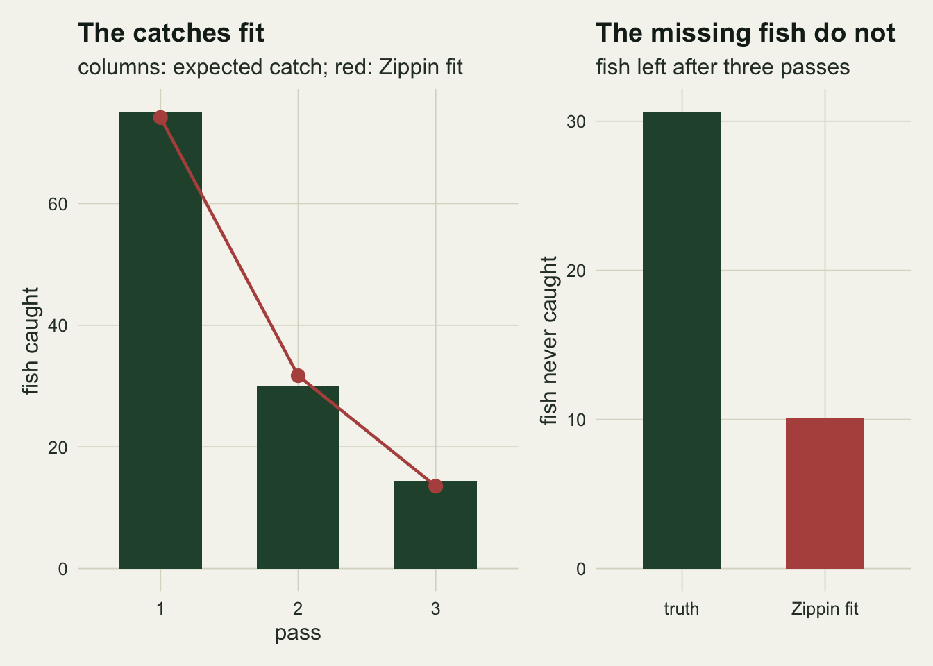
Bias and coverage over the design grid
The grid crosses three, four and five passes with first-pass catch probabilities of 0.3, 0.5 and 0.7 and per-pass multipliers of 1, 0.9, 0.8 and 0.6. Each of the 36 cells holds 300 simulated surveys, so a coverage near 0.95 carries a Monte Carlo standard error of about 0.013 and a coverage near one half about 0.029.
n_rep   <- 300
k_grid  <- c(3, 4, 5)
p1_grid <- c(0.3, 0.5, 0.7)
d_grid  <- c(1, 0.9, 0.8, 0.6)
cells   <- expand.grid(k = k_grid, p1 = p1_grid, d = d_grid)

set.seed(4417)
grid_res <- do.call(rbind, lapply(seq_len(nrow(cells)), function(i) {
  cm  <- sim_catch(n_rep, cells$k[i], cells$p1[i], cells$d[i])
  zp  <- zippin(cm)
  lr  <- profile_lr(cm)
  csn <- carle_strub(cm)
  wald_cover <- abs(zp$n_hat - n_true) / zp$se <= qnorm(0.975)
  data.frame(cells[i, ],
             fail      = mean(zp$fail),
             med_zip   = median(ifelse(zp$fail, Inf, zp$n_hat)) / n_true,
             med_cs    = median(csn) / n_true,
             cov_prof  = mean(lr[2, ] <= chi_cut),
             cov_wald  = mean(!is.na(wald_cover) & wald_cover),
             med_p_hat = median(zp$p_hat, na.rm = TRUE))
}))

cell_of <- function(k, p1, d) grid_res[grid_res$k == k & grid_res$p1 == p1 &
                                         grid_res$d == d, ]
c_const <- cell_of(3, 0.5, 1)
c_08    <- cell_of(3, 0.5, 0.8)
c_06    <- cell_of(3, 0.5, 0.6)
c_09    <- cell_of(3, 0.5, 0.9)
c_08_k4 <- cell_of(4, 0.5, 0.8)
c_08_k5 <- cell_of(5, 0.5, 0.8)
c_03    <- cell_of(3, 0.3, 1)
c_03_08 <- cell_of(3, 0.3, 0.8)
c_07_08 <- cell_of(3, 0.7, 0.8)
fail_max   <- max(grid_res$fail)
fail_cell  <- grid_res[which.max(grid_res$fail), ]
cs_zip_diff <- grid_res$med_zip - grid_res$med_cs
cs_below_all <- all(cs_zip_diff >= 0)
cs_zip_gap  <- max(cs_zip_diff)
cs_gap_cell <- grid_res[which.max(cs_zip_diff), ]
cs_gap_decl <- max(cs_zip_diff[grid_res$d < 1 & grid_res$p1 >= 0.5])
mc_se_95   <- sqrt(0.95 * 0.05 / n_rep)
mc_se_50   <- sqrt(0.25 / n_rep)
With constant catchability, three passes and a first-pass probability of 0.5, the median estimate is 0.999 of the true population, the profile interval covers in 0.930 of surveys and the Wald interval in 0.933. Both sit a little under 0.95, within two Monte Carlo standard errors of it (one standard error is 0.013 at that level), so with constant catchability the three-pass design behaves as the model promises.
A per-pass multiplier of 0.9 already pulls the median to 0.933 and the profile coverage to 0.700. At 0.8 the median is 0.868, the profile interval covers in 0.303 of surveys and the Wald interval in 0.200. At 0.6 the median is 0.743 and the two coverages are 0.000 and 0.000. The median catch probability estimated in the 0.8 cell is 0.577, against a true first-pass value of 0.5.
More passes do not rescue it. With a multiplier of 0.8 the median estimate is 0.886 with four passes and 0.895 with five, and the profile coverage falls to 0.093 and 0.037. Whatever the extra passes add, it does not move the centre up, and an interval around a centre that stays low reaches the truth less often. A low first-pass probability makes the bias larger: at 0.3 with a multiplier of 0.8 and three passes the median is 0.703, against 0.944 at 0.7. A high first-pass probability shrinks the bias but not the interval failure, since the profile coverage in that 0.7 cell is still only 0.260.
The Carle-Strub estimator gives no protection, and it was never meant to; its prior tames the infinite estimates of flat catch series, not a trend in catchability. Its median is at or below Zippin’s in every cell. The largest gap, 0.074 of the true population, is in the cell with 3 passes, a first-pass probability of 0.3 and constant catchability, where Carle-Strub itself sits below the truth at 0.947; with a declining catchability and a first-pass probability of 0.5 or more the two medians are never more than 0.013 apart. Infinite Zippin estimates were rare: the highest failure share in any cell is 0.007, in the cell with 3 passes, a first-pass probability of 0.3 and a multiplier of 1.0. Those surveys count as estimates of infinity in the medians and as failed Wald intervals in the coverage.
bias_long <- rbind(
  data.frame(grid_res[, c("k", "p1", "d")], median = grid_res$med_zip,
             estimator = "Zippin"),
  data.frame(grid_res[, c("k", "p1", "d")], median = grid_res$med_cs,
             estimator = "Carle-Strub"))
bias_long$passes <- factor(paste(bias_long$k, "passes"))
bias_long$p1_lab <- paste("first-pass p", bias_long$p1)

ggplot(bias_long, aes(d, median, colour = passes, linetype = estimator)) +
  geom_hline(yintercept = 1, colour = te_body, linewidth = 0.4) +
  geom_line(linewidth = 0.8) +
  geom_point(data = bias_long[bias_long$estimator == "Zippin", ], size = 2) +
  facet_wrap(~ p1_lab) +
  scale_colour_manual(values = c(te_gold, te_forest, te_rust), name = NULL) +
  scale_linetype_manual(values = c("Zippin" = "solid", "Carle-Strub" = "dotted"),
                        name = NULL) +
  scale_x_reverse(breaks = d_grid) +
  labs(x = "per-pass catchability multiplier (1 = constant)",
       y = "median estimate / true N",
       title = "Falling catchability, falling estimate",
       subtitle = "300 simulated surveys of 150 fish per point") +
  theme_datasheet() +
  theme(legend.position = "bottom", panel.spacing = unit(1.4, "lines"))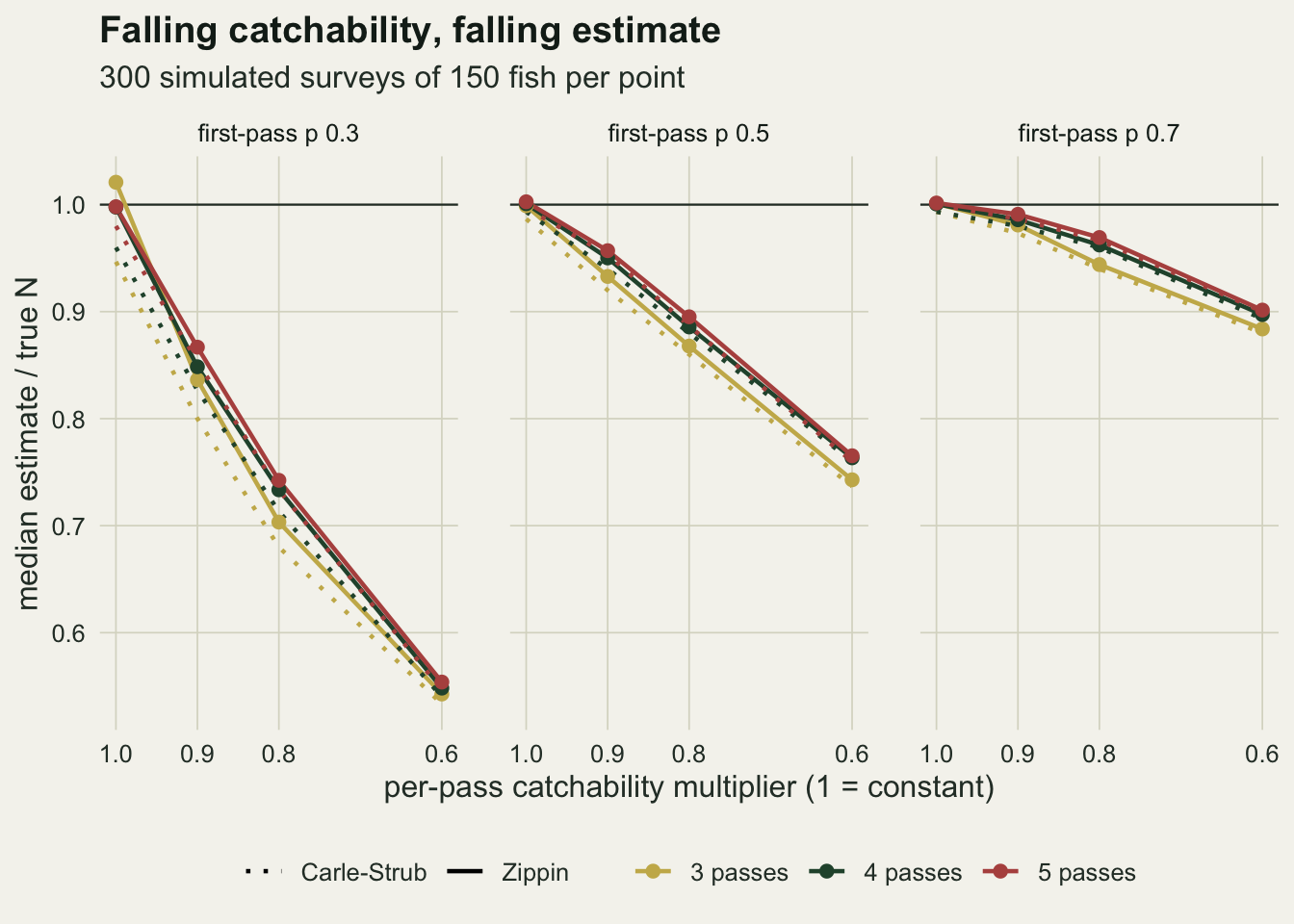
cov_long <- rbind(
  data.frame(grid_res[, c("k", "p1", "d")], coverage = grid_res$cov_prof,
             interval = "profile likelihood"),
  data.frame(grid_res[, c("k", "p1", "d")], coverage = grid_res$cov_wald,
             interval = "Wald"))
cov_long$passes <- factor(paste(cov_long$k, "passes"))
cov_long$p1_lab <- paste("first-pass p", cov_long$p1)

ggplot(cov_long, aes(d, coverage, colour = passes, linetype = interval)) +
  geom_hline(yintercept = 0.95, linetype = "dashed", colour = te_body,
             linewidth = 0.4) +
  geom_line(linewidth = 0.8) +
  geom_point(data = cov_long[cov_long$interval == "profile likelihood", ],
             size = 2) +
  facet_wrap(~ p1_lab) +
  scale_colour_manual(values = c(te_gold, te_forest, te_rust), name = NULL) +
  scale_linetype_manual(values = c("profile likelihood" = "solid", "Wald" = "dotted"),
                        name = NULL) +
  scale_x_reverse(breaks = d_grid) +
  scale_y_continuous(limits = c(0, 1)) +
  labs(x = "per-pass catchability multiplier (1 = constant)",
       y = "interval coverage",
       title = "The interval stops covering the truth",
       subtitle = "dashed line: nominal 0.95") +
  theme_datasheet() +
  theme(legend.position = "bottom", panel.spacing = unit(1.4, "lines"))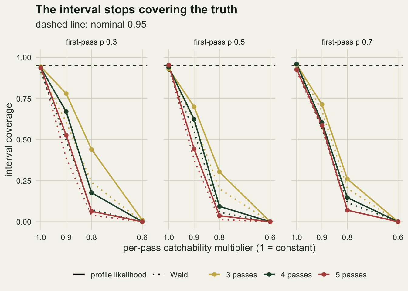
The goodness-of-fit test, calibrated
The obvious defence is to test the fit. Conditional on the total catch, the catches on the k passes are multinomial with probabilities proportional to p q^(j - 1), and a chi-square statistic on observed against expected catches has k - 2 degrees of freedom once p is estimated. With three passes that leaves one degree of freedom for detecting anything at all.
A chi-square reference distribution on 100 or so fish spread over three or four cells is an approximation, so its rejection rate under constant catchability is not guaranteed to be five per cent. Each survey is therefore also given a parametric bootstrap p-value: 199 catch series are drawn from the fitted multinomial with the same total, p is re-estimated on each, and the p-value is the share of bootstrap statistics at least as large as the observed one. Riley and Fausch already warned that this test is weak for small populations; the calibration below asks how weak. The fair question is not whether the test rejects in more than five per cent of surveys with a declining catchability, but whether it rejects more often than it does in the constant cell with the same passes and first-pass probability. This arm is cheap, so it uses 1000 surveys per cell instead of 300.
pi_matrix <- function(p, k) {
  q <- 1 - p
  m <- outer(q, 0:(k - 1), "^") * p
  m / (1 - q^k)
}
chi_gof <- function(catch_mat) {
  k     <- ncol(catch_mat)
  total <- rowSums(catch_mat)
  p_hat <- p_from_ratio(as.vector(catch_mat %*% (0:(k - 1))) / total, k)
  expct <- pi_matrix(p_hat, k) * total
  list(x2 = rowSums((catch_mat - expct)^2 / expct), p = p_hat, total = total)
}
boot_gof <- function(catch_mat, n_boot = 199) {
  k      <- ncol(catch_mat)
  n_surv <- nrow(catch_mat)
  obs    <- chi_gof(catch_mat)
  probs  <- pi_matrix(obs$p, k)[rep(seq_len(n_surv), each = n_boot), , drop = FALSE]
  left   <- rep(obs$total, each = n_boot)
  draws  <- matrix(0, length(left), k)
  used   <- 0
  for (j in seq_len(k - 1)) {
    x_j <- rbinom(length(left), left, pmin(1, probs[, j] / (1 - used)))
    draws[, j] <- x_j
    left <- left - x_j
    used <- used + probs[, j]
  }
  draws[, k] <- left
  boot_x2 <- matrix(chi_gof(draws)$x2, n_surv, byrow = TRUE)
  list(p_boot = (1 + rowSums(boot_x2 >= obs$x2)) / (n_boot + 1),
       p_chisq = pchisq(obs$x2, k - 2, lower.tail = FALSE))
}

n_gof <- 1000
set.seed(8830)
gof_res <- do.call(rbind, lapply(seq_len(nrow(cells)), function(i) {
  cm <- sim_catch(n_gof, cells$k[i], cells$p1[i], cells$d[i])
  bt <- boot_gof(cm)
  data.frame(cells[i, ], rej_chisq = mean(bt$p_chisq < 0.05),
             rej_boot = mean(bt$p_boot <= 0.05))
}))
gof_res$se_boot <- sqrt(gof_res$rej_boot * (1 - gof_res$rej_boot) / n_gof)
gof_of <- function(k, p1, d) gof_res[gof_res$k == k & gof_res$p1 == p1 &
                                       gof_res$d == d, ]
g3_1  <- gof_of(3, 0.5, 1);  g3_8 <- gof_of(3, 0.5, 0.8); g3_6 <- gof_of(3, 0.5, 0.6)
g4_1  <- gof_of(4, 0.5, 1);  g4_8 <- gof_of(4, 0.5, 0.8); g4_6 <- gof_of(4, 0.5, 0.6)
g5_1  <- gof_of(5, 0.5, 1);  g5_8 <- gof_of(5, 0.5, 0.8); g5_6 <- gof_of(5, 0.5, 0.6)
g5_7_8 <- gof_of(5, 0.7, 0.8); g5_7_6 <- gof_of(5, 0.7, 0.6); g3_7_8 <- gof_of(3, 0.7, 0.8)
g5_3_6 <- gof_of(5, 0.3, 0.6)
chisq_const_range <- range(gof_res$rej_chisq[gof_res$d == 1])
boot_const_range  <- range(gof_res$rej_boot[gof_res$d == 1])
k3_excess <- gof_res$rej_boot[gof_res$k == 3 & gof_res$d == 0.8] -
  gof_res$rej_boot[gof_res$k == 3 & gof_res$d == 1]
k3_excess_max <- max(k3_excess)
k3_excess_p1  <- gof_res$p1[gof_res$k == 3 & gof_res$d == 0.8][which.max(k3_excess)]
g3_max_1 <- gof_of(3, k3_excess_p1, 1); g3_max_8 <- gof_of(3, k3_excess_p1, 0.8)
k3_best_rej   <- max(gof_res$rej_boot[gof_res$k == 3 & gof_res$d < 1])
Under constant catchability the chi-square test rejects in between 0.034 and 0.064 of surveys across the nine combinations of passes and first-pass probability, and the bootstrap version in between 0.038 and 0.065. The Monte Carlo standard error of a rate near 0.05 from 1000 surveys is 0.007.
With three passes and a first-pass probability of 0.5, the bootstrap test rejects in 0.038 of surveys at constant catchability, 0.060 at a multiplier of 0.8 and 0.093 at 0.6, with Monte Carlo standard errors of about 0.008. At the multiplier of 0.8 the three-pass test gains at most 0.060 over its own constant-catchability rate in any of the three first-pass probabilities (the largest gain is with a first-pass probability of 0.7, from 0.055 to 0.115), and no three-pass cell with a declining catchability rejects in more than 0.177 of surveys. In the same design the profile interval missed the true population in 0.697 of surveys. The test is not strictly blind, but it rejects a handful of surveys where the interval fails in most of them.
Extra passes give the test something to work with. With a first-pass probability of 0.5 and four passes the bootstrap rejection rate goes from 0.052 at constant catchability to 0.094 at 0.8 and 0.169 at 0.6; with five passes from 0.049 to 0.110 and 0.208. The test does best when the first pass is efficient: with a first-pass probability of 0.7 and five passes it rejects 0.309 of surveys at 0.8 and 0.491 at 0.6, while three passes in the 0.7 and 0.8 cell reject 0.115. With a first-pass probability of 0.3 even five passes at 0.6 reject only 0.077, and that corner of the grid is where the estimates are lowest.
gof_plot <- gof_res
gof_plot$passes <- factor(paste(gof_plot$k, "passes"))
gof_plot$p1_lab <- paste("first-pass p", gof_plot$p1)

ggplot(gof_plot, aes(d, rej_boot, colour = passes)) +
  geom_hline(yintercept = 0.05, linetype = "dashed", colour = te_body,
             linewidth = 0.4) +
  geom_errorbar(aes(ymin = rej_boot - 2 * se_boot, ymax = rej_boot + 2 * se_boot),
                width = 0.02, linewidth = 0.5) +
  geom_line(linewidth = 0.8) +
  geom_point(size = 2) +
  facet_wrap(~ p1_lab) +
  scale_colour_manual(values = c(te_gold, te_forest, te_rust), name = NULL) +
  scale_x_reverse(breaks = d_grid) +
  scale_y_continuous(limits = c(0, 1)) +
  labs(x = "per-pass catchability multiplier (1 = constant)",
       y = "share of surveys rejected",
       title = "The fit test notices late",
       subtitle = "bars: two Monte Carlo standard errors; dashed: 0.05") +
  theme_datasheet() +
  theme(legend.position = "bottom", panel.spacing = unit(1.4, "lines"))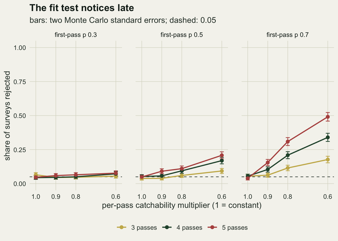
Modelling the decline with four or five passes
If catchability falls by a constant factor, why not put that factor in the model? The likelihood with p_j = p1 d^(j - 1) has three parameters, so it needs at least four passes to leave a degree of freedom. It is fitted below by maximum likelihood from three starting points, with a quasi-Newton polish of the best one, in the cells with a first-pass probability of 0.5. The profile likelihood ratio at N = 150 maximises over p1 and d with N held fixed. A fit counts as failed if the estimate exceeds twenty times the true population or the optimiser reports no convergence.
nll_decline <- function(x_row, n_val, p1, d_mult) {
  k   <- length(x_row)
  p_j <- p1 * d_mult^(0:(k - 1))
  if (any(p_j >= 1) || any(p_j <= 0) || !is.finite(n_val) || n_val > 1e9) return(1e10)
  remain <- n_val - c(0, cumsum(x_row)[-k])
  if (any(remain < x_row)) return(1e10)
  -sum(lchoose(remain, x_row) + x_row * log(p_j) + (remain - x_row) * log(1 - p_j))
}

fit_decline <- function(x_row) {
  total <- sum(x_row)
  f_three <- function(th) nll_decline(x_row, total + exp(th[1]), plogis(th[2]),
                                      exp(th[3]))
  starts <- list(c(log(20), 0, 0), c(log(100), -1, -0.2), c(log(5), 0.5, -0.5))
  fits   <- lapply(starts, function(s) optim(s, f_three, control = list(maxit = 2000)))
  best   <- fits[[which.min(vapply(fits, function(o) o$value, 0))]]
  polish <- optim(best$par, f_three, method = "BFGS")
  if (polish$value < best$value) best <- polish
  f_two <- function(th) nll_decline(x_row, n_true, plogis(th[1]), exp(th[2]))
  at_true <- min(optim(best$par[2:3], f_two)$value, optim(c(0, 0), f_two)$value)
  c(n_hat = total + exp(best$par[1]), d_hat = exp(best$par[3]),
    lr = 2 * (at_true - best$value), conv = best$convergence)
}

dec_cells <- expand.grid(k = c(4, 5), d = c(1, 0.8, 0.6))
set.seed(2291)
dec_res <- do.call(rbind, lapply(seq_len(nrow(dec_cells)), function(i) {
  cm   <- sim_catch(n_rep, dec_cells$k[i], 0.5, dec_cells$d[i])
  fits <- t(apply(cm, 1, fit_decline))
  bad  <- fits[, "n_hat"] > 20 * n_true | fits[, "conv"] != 0
  data.frame(dec_cells[i, ], fail = sum(bad),
             med_n = median(fits[, "n_hat"]) / n_true,
             cov   = mean(fits[, "lr"] <= chi_cut & !bad),
             d_q1  = quantile(fits[, "d_hat"], 0.25),
             d_med = median(fits[, "d_hat"]),
             d_q3  = quantile(fits[, "d_hat"], 0.75))
}))
dec_of <- function(k, d) dec_res[dec_res$k == k & dec_res$d == d, ]
dk4_8 <- dec_of(4, 0.8); dk4_6 <- dec_of(4, 0.6); dk5_8 <- dec_of(5, 0.8)
dk4_1 <- dec_of(4, 1);   dk5_6 <- dec_of(5, 0.6)
big_n   <- 150000
set.seed(7702)
big_row <- {
  left <- big_n; x_big <- numeric(4)
  for (j in 1:4) { x_big[j] <- rbinom(1, left, 0.5 * 0.8^(j - 1)); left <- left - x_big[j] }
  x_big
}
big_tot <- sum(big_row)
f_big   <- function(th) nll_decline(big_row, big_tot + exp(th[1]), plogis(th[2]), exp(th[3]))
big_fit <- optim(optim(c(log(big_n / 10), 0, 0), f_big, control = list(maxit = 5000))$par,
                 f_big, method = "BFGS")
big_n_ratio <- (big_tot + exp(big_fit$par[1])) / big_n
big_d_hat   <- exp(big_fit$par[3])
dec_fail_total <- sum(dec_res$fail)
dec_fits_total <- n_rep * nrow(dec_cells)
The decline model does not recover the population. With four passes and a true multiplier of 0.8 its median estimate is 0.870 of the truth, against 0.886 for Zippin on the same design, and at 0.6 it is 0.756. Five passes at 0.8 give 0.907. The estimated multiplier tells why: with four passes and a true value of 0.8, the middle half of the estimates runs from 0.91 to 1.17 around a median of 1.05, and with a true value of 0.6 the median is 0.99. Once more, a falling catchability in a population of 150 and a steadier one in a smaller population give catch series that four or five passes on this many fish cannot tell apart.
Its profile intervals cover more often than Zippin’s, 0.803 with four passes at 0.8 and 0.737 with five at 0.6, but still well short of 0.95, and even with constant catchability the four-pass coverage is 0.800. Failed fits numbered 0 out of 1800, so the problem is not the optimiser giving up; it is an answer the data cannot pin down. The model is identifiable in principle: fitted to one simulated reach of 150000 fish, a thousand times larger, with four passes and a multiplier of 0.8, it returns a multiplier of 0.768 and an estimate of 1.035 of the truth. On a reach of 150 fish the information is not there.
An efficiency release before the first pass
The repair adds information from outside the removal series. Before the first pass the crew releases M fin-clipped fish of the same species and size, caught elsewhere, lets them settle, and then runs the passes as usual, recording marked and unmarked fish separately. If the marked fish have the same catchability on every pass as the residents, including the decline, the share of marked fish caught over all passes estimates the overall capture probability directly, and the unmarked catch divided by that share estimates the population. The profile likelihood treats the unmarked total and the marked total as two binomial draws with the same capture probability.
release_fit <- function(tot_u, tot_m, m_rel) {
  ll <- function(nv, tu, tm) {
    p_c <- (tu + tm) / (nv + m_rel)
    lchoose(nv, tu) + (tu + tm) * log(p_c) + (nv - tu + m_rel - tm) * log(1 - p_c)
  }
  vapply(seq_along(tot_u), function(i) {
    top <- optimize(function(nv) ll(nv, tot_u[i], tot_m[i]),
                    c(tot_u[i], 50 * tot_u[i] + 500), maximum = TRUE)
    c(top$maximum, 2 * (top$objective - ll(n_true, tot_u[i], tot_m[i])))
  }, numeric(2))
}

n_rel_rep <- 1000
rel_cells <- expand.grid(m_rel = c(25, 50, 100), p1 = c(0.3, 0.5),
                         d = c(1, 0.8, 0.6))
set.seed(5163)
rel_res <- do.call(rbind, lapply(seq_len(nrow(rel_cells)), function(i) {
  p_j <- rel_cells$p1[i] * rel_cells$d[i]^(0:2)
  p_c <- 1 - prod(1 - p_j)
  tot_u <- rbinom(n_rel_rep, n_true, p_c)
  tot_m <- rbinom(n_rel_rep, rel_cells$m_rel[i], p_c)
  fit   <- release_fit(tot_u, tot_m, rel_cells$m_rel[i])
  data.frame(rel_cells[i, ], med_n = median(fit[1, ]) / n_true,
             cov = mean(fit[2, ] <= chi_cut))
}))
rel_se  <- sqrt(0.95 * 0.05 / n_rel_rep)
rel_of  <- function(m, p1, d) rel_res[rel_res$m_rel == m & rel_res$p1 == p1 &
                                        rel_res$d == d, ]
r50_8   <- rel_of(50, 0.5, 0.8); r25_8 <- rel_of(25, 0.5, 0.8)
r50_03  <- rel_of(50, 0.3, 0.6)
rel_cov_range_50 <- range(rel_res$cov[rel_res$m_rel >= 50])
rel_med_range_50 <- range(rel_res$med_n[rel_res$m_rel >= 50])

shy_factor <- 0.9
p_j_show   <- p1_show * d_show^(0:2)
p_c_res    <- 1 - prod(1 - p_j_show)
p_c_mark   <- 1 - prod(1 - shy_factor * p_j_show)
shy_ratio  <- p_c_res / p_c_mark

# individual heterogeneity: p ~ Beta(2, 2), constant per fish over three passes;
# release fish come from one electrofishing capture elsewhere, so selected with weight p
het_a <- 2; het_b <- 2
pc_ind   <- function(p) 1 - (1 - p)^3
het_res  <- integrate(function(p) pc_ind(p) * dbeta(p, het_a, het_b), 0, 1)$value
het_mark <- integrate(function(p) pc_ind(p) * p * dbeta(p, het_a, het_b), 0, 1)$value /
  (het_a / (het_a + het_b))
het_ratio <- het_res / het_mark
With 50 marked fish, three passes, a first-pass probability of 0.5 and a multiplier of 0.8, the median estimate is 0.987 of the true population and the profile interval covers in 0.939 of surveys, against 0.868 and 0.303 for Zippin on the same design. With 25 marked fish the numbers are 0.961 and 0.921. Across every cell with at least 50 marked fish the median estimate lies between 0.987 and 0.997 of the truth and the coverage between 0.931 and 0.959, with a Monte Carlo standard error of 0.007 near 0.95. The multiplier no longer matters, because the marked fish carry the decline with them. This is true by construction: the simulation gives marked and resident fish the same capture probability on every pass, so what this arm measures is how many marked fish the interval needs, not whether that assumption holds.
The price is an assumption moved, not removed. The release estimates the population of fish that behave like the marked ones. If handling and transport leave the marked fish slightly less catchable, say 90 per cent of the residents’ probability on every pass, the overall capture probability is 0.796 for residents and 0.749 for marked fish at the 0.5 and 0.8 design, and the estimate converges to 1.062 times the truth, now biased high. The opposite error comes from how release fish are usually obtained. If they are caught by electrofishing elsewhere and catchability varies between individuals, the release is weighted towards catchable fish. With individual probabilities drawn from a Beta(2, 2) distribution (mean 0.5, constant for each fish over three passes) and each fish entering the release with a chance equal to its own catch probability, the overall capture probability is 0.800 for residents and 0.886 for marked fish, and the estimate converges to 0.903 times the truth, biased low for the same reason the eradication post gives: the fish a crew catches easily are not a random sample. Peterson and colleagues measured efficiency with a release of marked fish and reported that their marking did not appear to change three-pass efficiency in their streams, which is evidence for their procedure, not a guarantee for someone else’s.
zip_cov <- grid_res[grid_res$k == 3 & grid_res$p1 %in% c(0.3, 0.5) &
                      grid_res$d %in% c(1, 0.8, 0.6), c("p1", "d", "cov_prof")]
compare_df <- rbind(
  data.frame(p1 = zip_cov$p1, d = zip_cov$d, coverage = zip_cov$cov_prof,
             method = "Zippin, no release"),
  data.frame(p1 = rel_res$p1, d = rel_res$d, coverage = rel_res$cov,
             method = paste("release of", rel_res$m_rel, "marked fish")))
compare_df$method <- factor(compare_df$method,
                            levels = c("Zippin, no release", "release of 25 marked fish",
                                       "release of 50 marked fish",
                                       "release of 100 marked fish"))
compare_df$p1_lab <- paste("first-pass p", compare_df$p1)

ggplot(compare_df, aes(d, coverage, colour = method)) +
  geom_hline(yintercept = 0.95, linetype = "dashed", colour = te_body,
             linewidth = 0.4) +
  geom_line(linewidth = 0.8) +
  geom_point(size = 2) +
  facet_wrap(~ p1_lab) +
  scale_colour_manual(values = c(te_rust, te_gold, te_forest, te_ink), name = NULL) +
  scale_x_reverse(breaks = c(1, 0.8, 0.6)) +
  scale_y_continuous(limits = c(0, 1)) +
  labs(x = "per-pass catchability multiplier (1 = constant)",
       y = "profile interval coverage",
       title = "Marked fish carry the decline with them",
       subtitle = "three passes, 150 fish; dashed: nominal 0.95") +
  theme_datasheet() +
  theme(legend.position = "bottom", panel.spacing = unit(1.4, "lines")) +
  guides(colour = guide_legend(nrow = 2))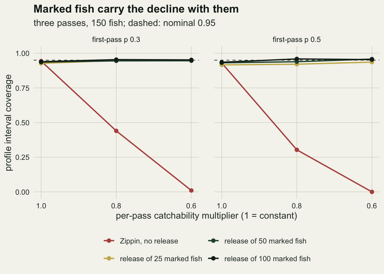
What to report
Report the catch on every pass, not only the estimate. The pass-by-pass numbers are what a reader needs to judge whether the decline is plausible, and they cost one line of a table.
Do not offer a passed goodness-of-fit test as evidence that catchability was constant. With three passes the test has one degree of freedom, and in these simulations its rejection rate at a multiplier of 0.8 rose by at most 0.060 above its constant-catchability rate, whichever first-pass probability was used, while the profile interval covered the truth in only 0.303 of surveys. If a test is reported, say whether its reference distribution was the chi-square or a bootstrap.
Treat a three-pass removal estimate as a lower bound unless catchability was checked independently. A multiplier of 0.8 lowered the median estimate to 0.868 of the truth, and adding a fourth or fifth pass or a decline parameter did not change that materially on a reach of 150 fish.
Where the estimate matters, budget for a check from outside the removal series: a release of marked fish before the first pass, or a reach where a mark-recapture estimate can be compared with the removal estimate. State how many marked fish were released, how they were caught, how they were handled and how long they settled, because the estimate is only as good as the claim that they behave like the residents.
Honest limits
The decline is a fixed geometric multiplier applied to every fish. Real declines come from at least two sources that behave differently: fish that learn or are stunned and hide after an escape, which is a behavioural response, and fish that were always hard to catch, which is individual heterogeneity. Heterogeneity produces a falling average catchability too, but the fish that remain are a filtered subset, as the eradication post shows, and the size of the bias depends on the spread of individual probabilities rather than on one multiplier. Nothing here separates those two sources, and apart from the closed-form release check in the section above, the numbers belong to the multiplier model only.
The multipliers were chosen as a grid, not taken from data. Riley and Fausch and Peterson and colleagues both found catchability falling over passes for stream salmonids, and Peterson and colleagues found a low first-pass efficiency as well, which is the corner of the grid where the bias here is largest. Their abstract reports a mean first-pass efficiency of 28 per cent that fell by a factor of 1.71 over successive passes, which puts their streams nearer the 0.3 and 0.6 corner than the 0.5 and 0.8 cell used as the example here. How steeply catchability falls depends on species, fish size, conductivity, habitat complexity and crew, and whether 0.8 is typical of a given stream is a question for that stream’s own calibration data. The post measures the consequence of each multiplier; it does not claim which one applies.
The population is 150 fish throughout. With a larger population the decline model becomes identifiable in principle, as the single fit to a reach a thousand times larger showed (a reach that size is not a practical survey), and the goodness-of-fit test should gain power as the expected counts grow, though no population size other than 150 was run through it. The conclusion that four or five passes cannot fix the problem is tied to reaches holding fish in the low hundreds, which is what many electrofishing reaches hold, but it is not a general statement.
The efficiency release was simulated in its most favourable form: marked fish mix fully, suffer no mortality, are always recognised and share the residents’ decline exactly. The two departures checked, a uniform ten per cent handling penalty and release fish selected by their own catchability from a Beta(2, 2) spread, were computed in closed form rather than simulated; the size of the second depends on that assumed spread and on a fish keeping its catchability when it is moved from the capture site to the reach. Real release trials also contend with marked fish leaving the reach or concentrating near the release point.
The Wald standard error uses the Zippin variance formula and fails whenever its denominator is not positive; those surveys were counted as intervals that missed. The profile interval was judged only by whether it contained N = 150, not by its width, so the comparison of the two intervals is a comparison of coverage alone.
References
Zippin C 1958 Journal of Wildlife Management 22(1):82-90 (10.2307/3797301)
Carle FL, Strub MR 1978 Biometrics 34(4):621-630 (10.2307/2530381)
Riley SC, Fausch KD 1992 North American Journal of Fisheries Management 12(4):768-776 (10.1577/1548-8675(1992)012<0768:UOTPSB>2.3.CO;2)
Peterson JT, Thurow RF, Guzevich JW 2004 Transactions of the American Fisheries Society 133(2):462-475 (10.1577/03-044)
Seber GAF 1982 The Estimation of Animal Abundance and Related Parameters, 2nd edition (Blackburn Press reprint 2002, ISBN 1-930665-55-5)