library(ggplot2)

te_paper  <- "#f5f4ee"
te_ink    <- "#16241d"
te_body   <- "#2c3a31"
te_forest <- "#275139"
te_rust   <- "#b5534e"
te_gold   <- "#c9b458"
te_line   <- "#dad9ca"

theme_datasheet <- function() {
  theme_minimal(base_size = 12) +
    theme(plot.background  = element_rect(fill = te_paper, colour = NA),
          panel.background = element_rect(fill = te_paper, colour = NA),
          panel.grid.major = element_line(colour = te_line, linewidth = 0.3),
          panel.grid.minor = element_blank(),
          text             = element_text(colour = te_body),
          plot.title       = element_text(colour = te_ink, face = "bold"),
          plot.subtitle    = element_text(colour = te_body),
          axis.text        = element_text(colour = te_body),
          strip.text       = element_text(colour = te_ink, face = "bold"))
}Camera trap occupancy: choosing the occasion length
R
occupancy
imperfect detection
camera traps
survey design
ecology tutorial
Daily occasions from a camera trap break the independence an occupancy model assumes. Measuring in R how the occasion length moves the bias and the coverage.
A hundred and fifty cameras go out along forest trails for thirty nights each, one camera per site, and the target is a pine marten. When the cards come back, the photographs have already been through the usual filter that turns bursts into events, and what is left for each camera is a string of thirty days, each one either a detection or not. The occupancy model wants repeat visits. The camera made one continuous visit. So the analyst has to cut it up, and the question that arrives in every lab meeting is whether each day is an occasion, or each week, and whether it matters.
It matters because of the animal, not the camera. A marten that is using a trail this week is likely to use it again tomorrow, and a marten that is working another part of its range is likely to stay away for a while. Consecutive days at an occupied camera are positively correlated. The single-season model assumes something else: given that a site is occupied, detections on different occasions are independent. Goldstein and colleagues 2024 examined exactly this for camera traps, by simulation and on 22 North American mammal species. The summary of their paper reports that temporal autocorrelation biases occupancy estimates and makes the model understate its uncertainty, that longer detection windows reduce the bias, and that a join count goodness-of-fit test detects the autocorrelation. This post is a small, base R demonstration of that result on one marten-like design, with the mechanism measured, the cost of the remedy measured, and the check written out so it can be run on real histories. None of it is new; the numbers are.
The likelihood itself is not re-derived here: fitting single-season occupancy models writes it out by hand and fits it with optim, and states the independence assumption this post breaks. How many visits? Occupancy survey design answers the sites against visits question when every visit is an independent trip; here the visits are carved out of one deployment, so cutting it finer adds occasions without adding independent information. Occupancy from unstructured records measures how the width of a visit window moves the estimate when visits are rebuilt from a record stream, where the dependence comes from recorders; here it comes from the animal. And checking a camera trap density estimate deals with the independence filter that turns a burst of photographs into one event, which works on the scale of minutes; everything below happens after that filter, on the scale of days.
A trail camera with a memory
Hines and colleagues 2010 built occupancy models for spatial replicates with Markovian dependence and applied them to a large-scale tiger survey on trails in Karnataka. They gave two models: an underlying Markov model for spatial dependence in the species’ local presence, and a trap-response model with Markovian detections. The simulation here uses the second, simpler structure with days in place of spatial replicates, nested inside ordinary site occupancy: the detection string at an occupied camera is the chain itself. At an occupied camera, a detection today follows a detection yesterday with probability 0.6 and follows a blank day with probability 0.05. The first day starts from the chain’s long-run distribution.
All design constants were fixed before anything ran: 150 sites, occupancy 0.5, 30 days, the two transition probabilities above, and one weaker setting for sensitivity, 0.3 after a detection and 0.08 after a blank.
n_site <- 150; psi_set <- 0.5; n_day <- 30
p11_set <- 0.6; p01_set <- 0.05; p11_weak <- 0.3; p01_weak <- 0.08
len_set <- c(1, 2, 3, 5, 10, 15)
p_stat <- p01_set / (1 - p11_set + p01_set)
p_weak <- p01_weak / (1 - p11_weak + p01_weak)
sim_days <- function(n_s, psi, n_t, p01, p11) {
  z_occ <- rbinom(n_s, 1, psi)
  y_day <- matrix(0L, n_s, n_t)
  p_st  <- p01 / (1 - p11 + p01)
  y_day[, 1] <- rbinom(n_s, 1, p_st) * z_occ
  for (tt in 2:n_t) {
    p_now <- ifelse(y_day[, tt - 1] == 1, p11, p01)
    y_day[, tt] <- rbinom(n_s, 1, p_now) * z_occ
  }
  y_day
}
blank_true  <- (1 - p_stat) * (1 - p01_set)^(n_day - 1)
blank_weak  <- (1 - p_weak) * (1 - p01_weak)^(n_day - 1)
blank_indep <- (1 - p_stat)^n_day
set.seed(4102)
n_chk <- 20000
y_chk <- sim_days(n_chk, 1, n_day, p01_set, p11_set)
blank_sim <- mean(rowSums(y_chk) == 0)
blank_se  <- sqrt(blank_sim * (1 - blank_sim) / n_chk)
rate_sim  <- mean(y_chk)
In the long run an occupied camera records the marten on a share 0.1111 of days, which is the transition probability after a blank divided by one minus the persistence plus that same probability; over 20000 simulated occupied cameras the observed daily rate is 0.1101. The difference from independent days is in how those detections are arranged. A run of detection days lasts on average one over one minus 0.6, which is 2.5 days, and the blank spells in between are long.
The quantity that decides everything later is the probability that an occupied camera records nothing in thirty days. Under the chain it has a closed form: a blank first day, then twenty-nine blank-to-blank steps, which gives 0.2008. The simulated cameras agree at 0.2032, with a Monte Carlo standard error of 0.0028. If the same daily rate fell on independent days, the chance of thirty blanks would be 0.0292. Same marginal rate, 6.9 times as many silent occupied cameras.
set.seed(4103)
n_show <- 20
y_mk_show <- sim_days(n_show, 1, n_day, p01_set, p11_set)
y_in_show <- sim_days(n_show, 1, n_day, p_stat, p_stat)
as_tiles <- function(y, lab) data.frame(site = as.vector(row(y)), day = as.vector(col(y)),
                                        det = as.vector(y), kind = lab)
tile_df <- rbind(as_tiles(y_mk_show, "trail use persists (0.6 after a detection)"),
                 as_tiles(y_in_show, "independent days, same daily rate"))
tile_df$kind <- factor(tile_df$kind, levels = unique(tile_df$kind))
ggplot(tile_df, aes(day, site, fill = factor(det))) +
  geom_tile(colour = te_paper, linewidth = 0.4) +
  facet_wrap(~kind, ncol = 1) +
  scale_fill_manual(values = c("0" = te_line, "1" = te_forest),
                    labels = c("no detection", "detection"), name = NULL) +
  scale_x_continuous(breaks = c(1, 10, 20, 30), expand = c(0, 0)) +
  scale_y_continuous(breaks = NULL, expand = c(0, 0)) +
  labs(x = "camera day", y = "occupied camera",
       title = "Same detection rate, different arrangement",
       subtitle = "every camera here is occupied") +
  theme_datasheet() +
  theme(legend.position = "bottom", panel.grid.major = element_blank())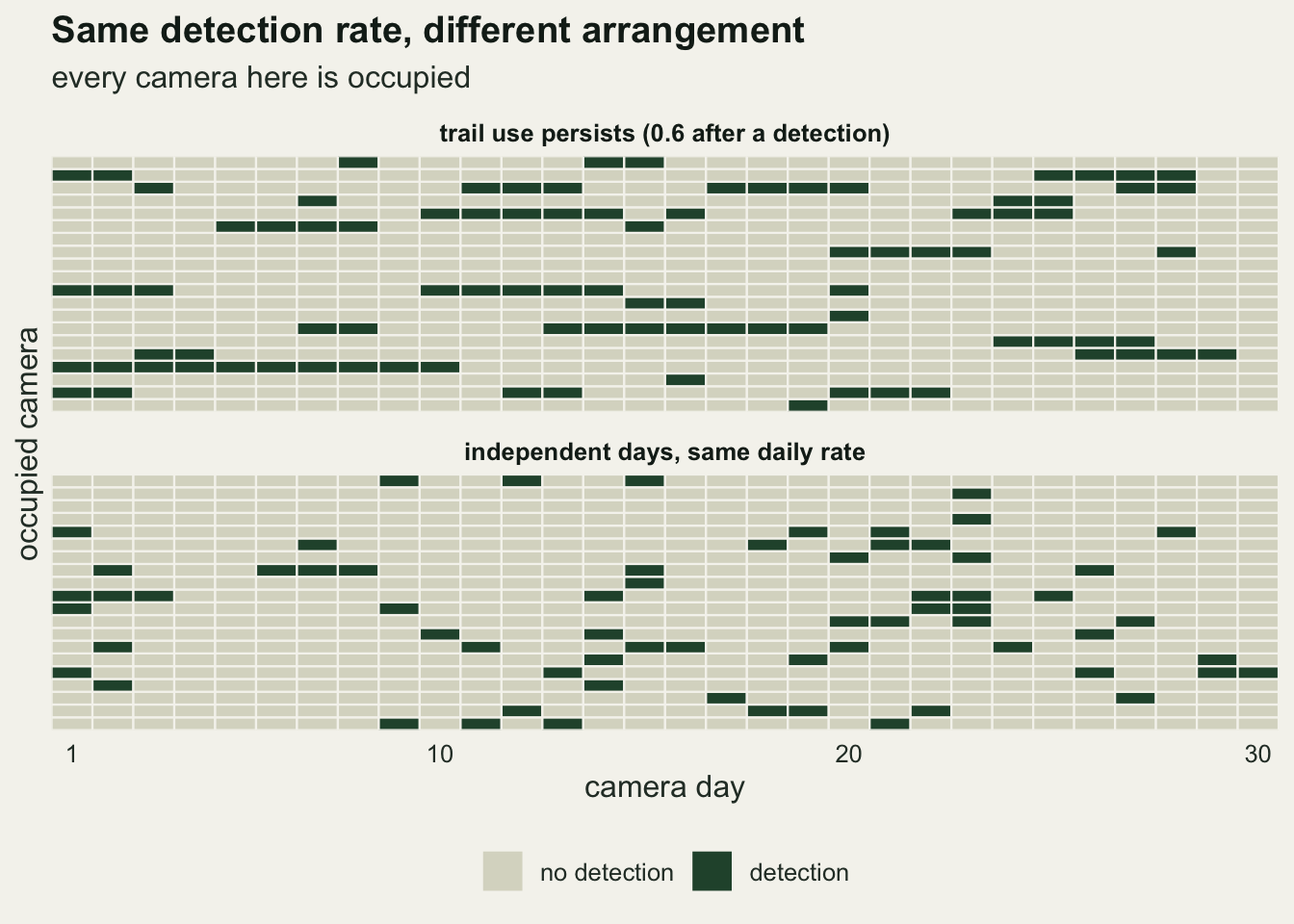
Daily occasions: the estimate falls short and the interval misses
Each simulated survey is cut into occasions of 1, 2, 3, 5, 10, 15 days, an occasion counting as a detection if the marten was seen on any day in it, and the standard constant occupancy, constant detection model is fitted to every version. The fit keeps the better of two starting points, one taken from the data and one fixed at the centre of the logit scale. The interval is the usual Wald interval on the logit scale, back-transformed. The control uses the same daily rate, 0.1111, with independent days: if the trouble is autocorrelation, the control must come out clean.
keep_in <- function(x) pmin(pmax(x, 0.02), 0.98)
nll_std <- function(th, n_d, k) {
  psi <- plogis(th[1]); p <- plogis(th[2]); d_seq <- 0:k
  lik <- psi * p^d_seq * (1 - p)^(k - d_seq)
  lik[1] <- lik[1] + 1 - psi
  -sum(n_d * log(lik))
}
fit_std <- function(y_occ) {
  k <- ncol(y_occ); d_site <- rowSums(y_occ); n_d <- tabulate(d_site + 1, k + 1)
  st_data <- qlogis(keep_in(c(mean(d_site > 0), mean(d_site[d_site > 0]) / k)))
  f_data  <- optim(st_data, nll_std, n_d = n_d, k = k, method = "BFGS", hessian = TRUE)
  f_fixed <- optim(c(0, 0), nll_std, n_d = n_d, k = k, method = "BFGS", hessian = TRUE)
  f_best  <- if (f_fixed$value < f_data$value) f_fixed else f_data
  se_l <- tryCatch(sqrt(diag(solve(f_best$hessian)))[1], error = function(e) NA_real_)
  c(psi = plogis(f_best$par[1]), p = plogis(f_best$par[2]), lpsi = f_best$par[1],
    se = se_l, gap = f_fixed$value - f_data$value, naive = mean(d_site > 0),
    psi_fx = plogis(f_fixed$par[1]), p_fx = plogis(f_fixed$par[2]), conv_fx = f_fixed$convergence)
}
collapse_days <- function(y_day, len) {
  grp <- rep(seq_len(ncol(y_day) / len), each = len)
  (t(rowsum(t(y_day), grp)) > 0) * 1L
}
n_rep <- 400
run_scenario <- function(p01, p11, seed) {
set.seed(seed)
out <- array(NA_real_, c(n_rep, length(len_set), 9),
dimnames = list(NULL, len_set, c("psi", "p", "lpsi", "se", "gap", "naive",
"psi_fx", "p_fx", "conv_fx")))
for (r in seq_len(n_rep)) {
y_day <- sim_days(n_site, psi_set, n_day, p01, p11)
for (j in seq_along(len_set)) out[r, j, ] <- fit_std(collapse_days(y_day, len_set[j]))
}
out
}
res_mk <- run_scenario(p01_set, p11_set, 5101)
res_in <- run_scenario(p_stat, p_stat, 5102)
res_wk <- run_scenario(p01_weak, p11_weak, 5103)
summ <- function(res) {
lo <- plogis(res[, , "lpsi"] - 1.96 * res[, , "se"])
hi <- plogis(res[, , "lpsi"] + 1.96 * res[, , "se"])
k_mat <- matrix(n_day / len_set, n_rep, length(len_set), byrow = TRUE)
data.frame(len = len_set, mean_psi = colMeans(res[, , "psi"]),
sd_psi = apply(res[, , "psi"], 2, sd), width = colMeans(hi - lo, na.rm = TRUE),
cover = colMeans(lo <= psi_set & hi >= psi_set, na.rm = TRUE),
n_na = colSums(is.na(res[, , "se"])), blank_fit = colMeans((1 - res[, , "p"])^k_mat))
}
s_mk <- summ(res_mk); s_in <- summ(res_in); s_wk <- summ(res_wk)
mc_cov <- sqrt(0.95 * 0.05 / n_rep)
bias_se_mk <- s_mk$sd_psi / sqrt(n_rep)
gap_all <- c(res_mk[, , "gap"], res_in[, , "gap"], res_wk[, , "gap"])
n_na_all <- sum(s_mk$n_na, s_in$n_na, s_wk$n_na)
res_all <- list(res_mk, res_in, res_wk)
bad_by_len <- Reduce(`+`, lapply(res_all, function(r) colSums(r[, , "gap"] > 0.01)))
pick_bad <- function(q) unlist(lapply(res_all, function(r) r[, , q][r[, , "gap"] > 0.01]))
psi_fx_bad <- pick_bad("psi_fx"); p_fx_bad <- pick_bad("p_fx"); conv_fx_bad <- pick_bad("conv_fx")With daily occasions the trail-use survey returns a mean occupancy estimate of 0.405 against a true 0.5, and the nominal 95 per cent interval contains the truth in 36.2 per cent of surveys. Widening the occasion moves both in the right direction: at five days the estimate is 0.451 with coverage 81.8 per cent, at ten days 0.474 and 91.8 per cent, at fifteen days 0.486 and 94.2 per cent. The Monte Carlo standard error of a coverage near 95 per cent is 1.1 percentage points, and that of the mean estimate at fifteen days is 0.0028, so at two occasions of fifteen days the estimate is still short by 5.1 of its Monte Carlo standard errors while the coverage sits 0.7 standard errors below nominal.
The control is clean. With independent days at the same daily rate the mean estimate at daily occasions is 0.496 and coverage is 97.2 per cent; across all six occasion lengths the mean stays within 0.0040 of the truth and the coverage between 96.2 and 97.8 per cent, on the safe side of nominal. The daily rate is the same, the number of cameras is the same, the model is the same. The only thing removed is the memory, and the bias goes with it.
The weaker setting, 0.3 after a detection and 0.08 after a blank, gives a daily rate of 0.1026 and a milder version of the same picture: 0.477 with coverage 92.0 per cent at daily occasions, 0.502 and 94.5 per cent at fifteen days.
Two checks on the fitting. Of 7200 fits, the fixed start ended with a worse likelihood than the data start in 765 (419 with daily occasions, 345 with two-day and 1 with three-day occasions, none at the longer lengths) and the reverse happened in 0. Those failures are not a second peak in the likelihood. The fixed start runs off towards occupancy one: its occupancy estimate was within \(4.0 \times 10^{-5}\) of one in every failure, with a detection probability between 0.035 and 0.148, and optim reported convergence every time, because on the logit scale the gradient in the occupancy direction vanishes as the estimate approaches one. A single fixed start at the centre of the logit scale is not safe with thirty occasions and a daily rate near a tenth. The Hessian was invertible in every fit.
scen_lab <- c("trail use, 0.6 after a detection", "weaker, 0.3 after a detection",
              "independent days (control)")
q_lab <- c("mean occupancy estimate", "95 per cent interval coverage")
long_q <- function(s, lab) {
  data.frame(len = s$len, value = c(s$mean_psi, s$cover),
             half = 1.96 * c(s$sd_psi / sqrt(n_rep), rep(mc_cov, length(s$len))),
             quantity = rep(q_lab, each = length(s$len)), scen = lab)
}
bias_df <- rbind(long_q(s_mk, scen_lab[1]), long_q(s_wk, scen_lab[2]), long_q(s_in, scen_lab[3]))
bias_df$scen <- factor(bias_df$scen, levels = scen_lab)
bias_df$quantity <- factor(bias_df$quantity, levels = q_lab)
ref_df <- data.frame(quantity = factor(q_lab, levels = q_lab), yint = c(psi_set, 0.95))
ggplot(bias_df, aes(len, value, colour = scen)) +
  geom_hline(data = ref_df, aes(yintercept = yint), linetype = "dashed",
             colour = te_body, linewidth = 0.6) +
  geom_errorbar(aes(ymin = value - half, ymax = value + half), width = 0.4, linewidth = 0.5) +
  geom_line(linewidth = 0.9) + geom_point(size = 2.2) +
  facet_wrap(~quantity, ncol = 2, scales = "free_y") +
  scale_colour_manual(values = c(te_rust, te_gold, te_forest), name = NULL) +
  scale_x_continuous(breaks = len_set) +
  guides(colour = guide_legend(nrow = 3)) +
  labs(x = "occasion length (days)", y = NULL,
       title = "Longer occasions pull the estimate back",
       subtitle = "dashed: the true occupancy and the nominal coverage; bars: 1.96 Monte Carlo SE") +
  theme_datasheet() + theme(legend.position = "bottom")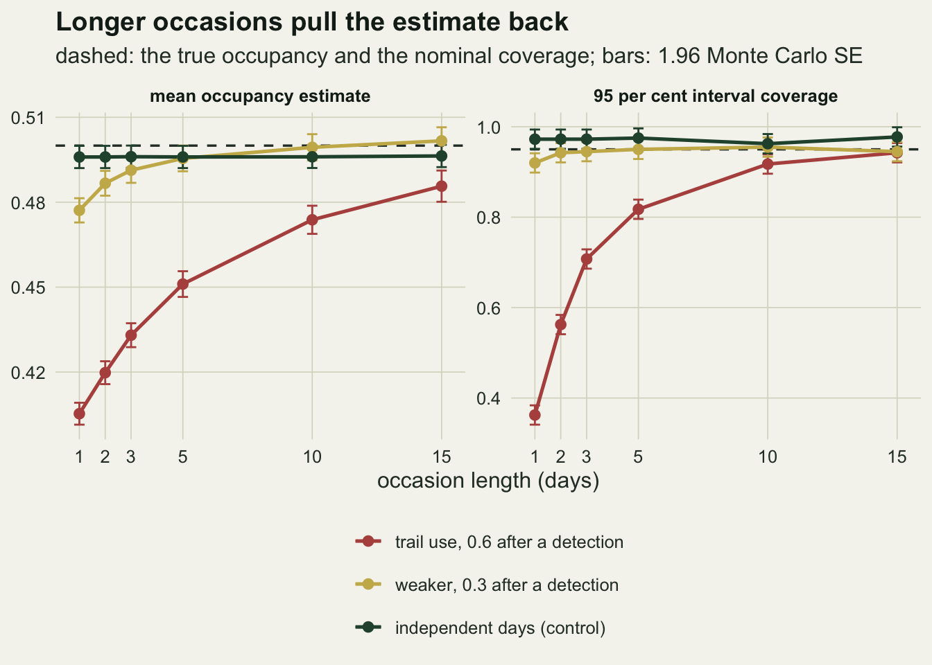
Why: the model thinks a silent month is almost impossible
The mechanism can be read off the fitted model. For the constant-detection model the maximum likelihood estimate satisfies an exact identity: setting the score for occupancy to zero gives estimated occupancy times one minus the fitted probability of an all-blank history equal to the share of cameras with at least one detection. So the estimate is the naive share divided by one minus the fitted blank probability, and every systematic error in occupancy is an error in that fitted blank probability.
ident_err <- max(abs(res_mk[, , "psi"] * (1 - (1 - res_mk[, , "p"])^
                   rep(n_day / len_set, each = n_rep)) - res_mk[, , "naive"]))
naive_mk   <- mean(res_mk[, 1, "naive"])
pred_psi_1 <- naive_mk / (1 - s_mk$blank_fit[1])
cor_day <- cor(as.vector(y_chk[, -n_day]), as.vector(y_chk[, -1]))
blank_fit_1 <- (1 - res_mk[, 1, "p"])^n_day
occ_blank_fit  <- mean(res_mk[, 1, "psi"] * blank_fit_1 /
                         (res_mk[, 1, "psi"] * blank_fit_1 + 1 - res_mk[, 1, "psi"]))
occ_blank_true <- psi_set * blank_true / (psi_set * blank_true + 1 - psi_set)
y_chk15 <- collapse_days(y_chk, 15)
cor_15  <- cor(y_chk15[, 1], y_chk15[, 2])
The identity holds in every fit to within \(9.44 \times 10^{-5}\). The share of cameras with a detection averages 0.4002, against its expectation of 0.3996, which is the true occupancy times one minus the true blank probability. The truth divides that share by one minus 0.2008 and gets back to 0.5.
The model at daily occasions divides by something else. It sees detection days arriving in runs at the cameras where the marten was found, so it fits a daily detection probability of 0.1388, above the long-run rate of 0.1111, and under independence that probability makes thirty blank days nearly impossible: the fitted blank probability averages 0.0125, while the truth is 0.2008, 16 times larger. The model concludes that almost every silent camera is empty: its implied share of occupied cameras among the silent ones averages 0.0085, where the truth is 0.1672. Dividing the naive share by one minus the fitted value gives 0.4053, against a mean estimate of 0.4053: the bias is the blank probability and nothing else.
Longer occasions help because a window of many days absorbs most of a run. Two occasions of fifteen days see only whether each half-month had any detection, and on the 20000 occupied cameras simulated earlier the correlation between the two occasions is 0.050, against 0.549 between consecutive days (for a two-state chain the lag one correlation is the difference of the two transition probabilities, 0.55). The fitted blank probability climbs to 0.1726, still short of the truth. The control makes the other half of the argument: with independent days the fitted blank probability is 0.0296 at daily occasions against a true 0.0292.
blank_df <- data.frame(len = len_set, fit = c(s_mk$blank_fit, s_wk$blank_fit, s_in$blank_fit),
                       truth = rep(c(blank_true, blank_weak, blank_indep), each = length(len_set)),
                       scen = factor(rep(scen_lab, each = length(len_set)), levels = scen_lab))
ggplot(blank_df, aes(len, fit, colour = scen)) +
  geom_hline(aes(yintercept = truth, colour = scen), linetype = "dashed", linewidth = 0.6) +
  geom_line(linewidth = 0.9) + geom_point(size = 2.2) +
  scale_colour_manual(values = c(te_rust, te_gold, te_forest), name = NULL) +
  scale_x_continuous(breaks = len_set) +
  scale_y_log10(breaks = c(0.01, 0.02, 0.05, 0.1, 0.2)) +
  guides(colour = guide_legend(nrow = 3)) +
  labs(x = "occasion length (days)", y = "P(no detection in 30 days | occupied)",
       title = "The blank probability is what goes wrong",
       subtitle = "solid: mean fitted value; dashed: the true value, same colour") +
  theme_datasheet() + theme(legend.position = "bottom")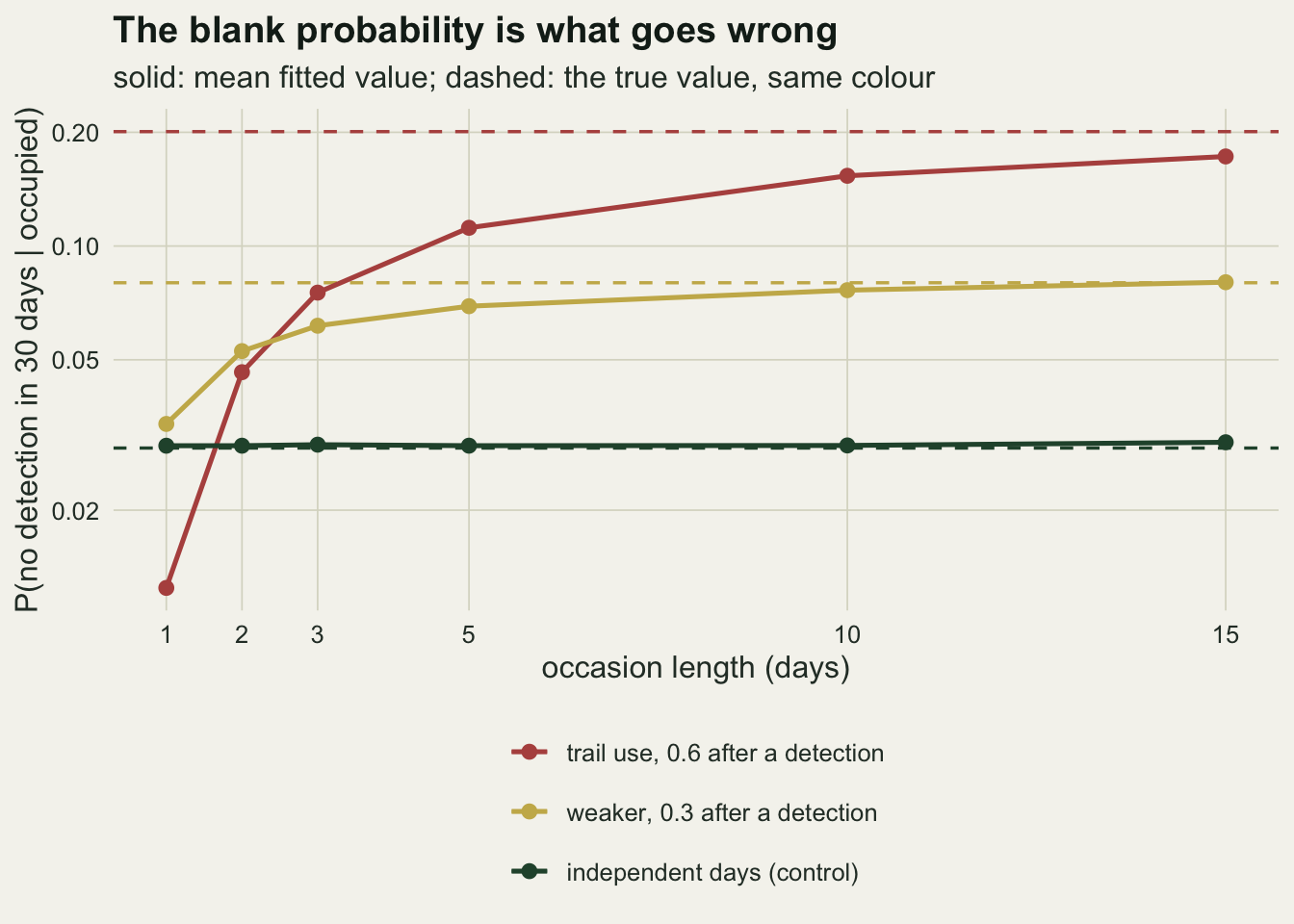
Fitting the dependence instead
Wider occasions are a workaround. The model-based fix is to write the dependence into the likelihood, as Hines and colleagues did for trails. In the trap-response form simulated here the likelihood of an occupied camera’s history is the chain’s probability of that exact string: the long-run probability for the first day, then one transition probability per day. It depends on the data only through the first day and the counts of the four kinds of day-to-day transition. A camera with no detection is a mixture, as in the standard model: occupied with a blank chain, or empty.
mk_stats <- function(y_day) {
  is_det <- rowSums(y_day) > 0; y_d <- y_day[is_det, , drop = FALSE]
  a_prev <- y_d[, -ncol(y_d)]; b_next <- y_d[, -1]
  c(n_det = sum(is_det), n_blank = sum(!is_det), first1 = sum(y_d[, 1]), first0 = sum(1 - y_d[, 1]),
    n01 = sum(a_prev == 0 & b_next == 1), n00 = sum(a_prev == 0 & b_next == 0),
    n11 = sum(a_prev == 1 & b_next == 1), n10 = sum(a_prev == 1 & b_next == 0))
}
nll_mk <- function(th, st, n_t) {
  psi <- plogis(th[1]); p01 <- plogis(th[2]); p11 <- plogis(th[3])
  p_st <- p01 / (1 - p11 + p01)
  ll_det <- st[["n_det"]] * log(psi) + st[["first1"]] * log(p_st) + st[["first0"]] * log(1 - p_st) +
    st[["n01"]] * log(p01) + st[["n00"]] * log(1 - p01) +
    st[["n11"]] * log(p11) + st[["n10"]] * log(1 - p11)
  ll_blank <- st[["n_blank"]] * log(psi * (1 - p_st) * (1 - p01)^(n_t - 1) + 1 - psi)
  -(ll_det + ll_blank)
}
fit_mk <- function(y_day) {
  st <- mk_stats(y_day)
  st_data <- qlogis(keep_in(c(st[["n_det"]] / nrow(y_day),
                              st[["n01"]] / (st[["n01"]] + st[["n00"]]),
                              st[["n11"]] / max(1, st[["n11"]] + st[["n10"]]))))
  f_data  <- optim(st_data, nll_mk, st = st, n_t = ncol(y_day), method = "BFGS", hessian = TRUE)
  f_fixed <- optim(c(0, -2, 0), nll_mk, st = st, n_t = ncol(y_day), method = "BFGS", hessian = TRUE)
  f <- if (f_fixed$value < f_data$value) f_fixed else f_data
  se_l <- tryCatch(sqrt(diag(solve(f$hessian)))[1], error = function(e) NA_real_)
  c(psi = plogis(f$par[1]), lpsi = f$par[1], se = se_l,
    p01 = plogis(f$par[2]), p11 = plogis(f$par[3]),
    gap = abs(f_fixed$value - f_data$value), naive = st[["n_det"]] / nrow(y_day))
}
set.seed(5101)
res_fix <- t(vapply(seq_len(n_rep), function(r)
  fit_mk(sim_days(n_site, psi_set, n_day, p01_set, p11_set)), numeric(7)))
stopifnot(all(res_fix[, "naive"] == res_mk[, 1, "naive"]))
lo_mk <- plogis(res_fix[, "lpsi"] - 1.96 * res_fix[, "se"])
hi_mk <- plogis(res_fix[, "lpsi"] + 1.96 * res_fix[, "se"])
mk_mean <- mean(res_fix[, "psi"]); mk_sd <- sd(res_fix[, "psi"])
mk_cover <- mean(lo_mk <= psi_set & hi_mk >= psi_set, na.rm = TRUE)
mk_width <- mean(hi_mk - lo_mk, na.rm = TRUE)
The seed is the one the trail-use scenario used, and the chunk checks survey by survey that the naive shares match those of the 400 trail-use surveys. At daily resolution the dependent model returns a mean occupancy estimate of 0.503 (Monte Carlo standard error 0.0028), coverage of 96.5 per cent, and mean transition estimates of 0.050 and 0.601 against the true 0.05 and 0.6; its two starting points reached different optima in 0 of the fits. It works because it is the true model here. A camera also misses animals that did walk past, and then the chain sits in a hidden local-presence state with a detection probability on top, which is the other form Hines and colleagues gave.
What long occasions cost
The obvious worry about collapsing thirty days into two occasions is precision. Measured against the model that is actually correct, that worry is small.
The spread of the occupancy estimate across surveys is 0.0563 with fifteen-day occasions, 0.0507 with ten-day occasions and 0.0556 for the dependent model at daily resolution: ratios of 1.01 and 0.91. The mean interval width at fifteen days is 0.224 against 0.222. The comparison that looks alarming is against independent days, where daily occasions give a spread of only 0.0401; but that precision was never on offer, because a marten that keeps returning to the same trail simply carries less information per day than one that turns up at random. Daily occasions under autocorrelation do not recover it either. They report an interval of 0.157 around the wrong centre.
The real cost of long occasions is in the detection model. A covariate that changes from day to day, a night’s temperature or rain, a lure that was refreshed, can enter a daily occasion as it is, but a fifteen-day occasion can carry only its average over the window. To measure what that loses, the next chunk switches the memory off (independent days, so the occupancy part of the standard model is right at every occasion length) and gives daily detection a logit slope of 0.5 on a standardised daily covariate, drawn separately for every camera and day. The slope is then estimated at occasions of one, five and fifteen days, with the window mean of the covariate as the occasion covariate.
nll_cov <- function(th, y_occ, w_occ) {
  psi <- plogis(th[1]); p <- plogis(th[2] + th[3] * w_occ)
  lp_hist <- rowSums(y_occ * log(p) + (1 - y_occ) * log(1 - p))
  is_det <- rowSums(y_occ) > 0
  -(sum(log(psi) + lp_hist[is_det]) + sum(log(psi * exp(lp_hist[!is_det]) + 1 - psi)))
}
window_mean <- function(w_day, len)
  t(rowsum(t(w_day), rep(seq_len(ncol(w_day) / len), each = len))) / len
b_cov <- 0.5; len_cov <- c(1, 5, 15); n_cov <- 200
set.seed(6203)
cov_res <- replicate(n_cov, {
  z_occ <- rbinom(n_site, 1, psi_set)
  w_day <- matrix(rnorm(n_site * n_day), n_site, n_day)
  y_day <- matrix(rbinom(n_site * n_day, 1, z_occ * plogis(qlogis(p_stat) + b_cov * w_day)),
                  n_site, n_day)
  vapply(len_cov, function(len) {
    y_occ <- collapse_days(y_day, len); w_occ <- window_mean(w_day, len)
    p_start <- min(0.9, mean(y_occ[rowSums(y_occ) > 0, ]))
    f <- optim(c(0, qlogis(p_start), 0), nll_cov, y_occ = y_occ, w_occ = w_occ,
               method = "BFGS", hessian = TRUE)
    se_b <- sqrt(diag(solve(f$hessian)))[3]
    c(b = f$par[3], z = f$par[3] / se_b, sd_w = sd(as.vector(w_occ)))
  }, numeric(3))
})
pow_cov <- rowMeans(abs(cov_res[2, , ]) > qnorm(0.975))
pow_se  <- sqrt(pow_cov * (1 - pow_cov) / n_cov)
b_mean <- rowMeans(cov_res[1, , ]); z_mean <- rowMeans(cov_res[2, , ])
sdw_mean <- rowMeans(cov_res[3, , ])
With daily occasions the covariate effect is detected (two-sided, five per cent) in 100.0 per cent of 200 surveys, with a mean z statistic of 7.4 and a mean slope of 0.497. With five-day occasions the detection rate falls to 89.0 per cent and with fifteen-day occasions to 22.5 per cent (Monte Carlo standard errors up to 3.0 points). The reason is visible in the covariate itself: averaging a daily variable over the window shrinks its spread from 1.000 to 0.446 and 0.258, so there is little left to regress on. That shrinkage is a closed form, not a finding: the mean of n independent standard normal days has standard deviation one over the square root of n, 0.447 for five days and 0.258 for fifteen, and the measured spreads above are the check. The slope also changes meaning, to 0.653 and 1.072 on average, because it now describes the detection of a whole window against the window mean, and it cannot be compared with a daily effect.
A check to run on your own histories
The first thing to look at needs nothing but the detection matrix. Among cameras with at least one detection, compare the share of days with a detection after a detection day and after a blank day. Independence given occupancy says they should be nearly equal: restricting to cameras with at least one detection nudges the rate after a blank day slightly up, and the shuffle below takes care of that exactly.
cond_rates <- function(y_day) {
  y_d <- y_day[rowSums(y_day) > 0, , drop = FALSE]
  a_prev <- y_d[, -ncol(y_d)]; b_next <- y_d[, -1]
  c(after_det = mean(b_next[a_prev == 1]), after_blank = mean(b_next[a_prev == 0]))
}
joins <- function(y_d) sum(y_d[, -ncol(y_d)] * y_d[, -1])
day_var <- function(y_d) var(colSums(y_d))
perm_stats <- function(y_d, n_perm) {
  n_r <- nrow(y_d); n_c <- ncol(y_d); v_row <- as.vector(t(y_d))
  key_row <- rep(seq_len(n_r), each = n_c)
  vapply(seq_len(n_perm), function(i) {
    y_perm <- matrix(v_row[order(key_row + runif(n_r * n_c))], n_r, n_c, byrow = TRUE)
    c(joins(y_perm), day_var(y_perm))
  }, numeric(2))
}
join_test <- function(y_day, n_perm) {
  y_d <- y_day[rowSums(y_day) > 0, , drop = FALSE]
  null <- perm_stats(y_d, n_perm); obs <- joins(y_d)
  list(obs = obs, null = null[1, ], p = (1 + sum(null[1, ] >= obs)) / (n_perm + 1),
       p_day = (1 + sum(null[2, ] >= day_var(y_d))) / (n_perm + 1))
}
sim_het <- function(n_s, psi, n_t, a_beta, b_beta) {
  z_occ <- rbinom(n_s, 1, psi); p_site <- rbeta(n_s, a_beta, b_beta)
  matrix(rbinom(n_s * n_t, 1, p_site * z_occ), n_s, n_t)
}
a_het <- 0.5; b_het <- a_het * (1 - p_stat) / p_stat
set.seed(7301)
y_ex_mk  <- sim_days(n_site, psi_set, n_day, p01_set, p11_set)
y_ex_in  <- sim_days(n_site, psi_set, n_day, p_stat, p_stat)
y_ex_het <- sim_het(n_site, psi_set, n_day, a_het, b_het)
cr_mk <- cond_rates(y_ex_mk); cr_in <- cond_rates(y_ex_in); cr_het <- cond_rates(y_ex_het)
n_perm_ex <- 999
jt_mk <- join_test(y_ex_mk, n_perm_ex); jt_in <- join_test(y_ex_in, n_perm_ex)
jt_het <- join_test(y_ex_het, n_perm_ex)
On one simulated survey of each kind, the trail-use cameras detect the marten on 0.583 of days after a detection day and on 0.057 after a blank day. Independent days give 0.097 and 0.120. That looks like a clean test, but it is not specific. A third survey has independent days and no memory at all, but cameras differ in how often they catch the marten: each site’s daily probability is drawn from a beta distribution with mean 0.1111 and first shape 0.5. It gives 0.336 after a detection and 0.139 after a blank, because the good cameras supply most of the detection days that are followed by another detection. Pooled over cameras, the comparison mixes the two causes.
The join count separates them. Count, over the detected cameras, the pairs of consecutive days that both hold a detection, then shuffle the days within each camera many times and count again. Shuffling within a camera keeps every camera’s number of detection days, so between-camera differences survive it and only the order is destroyed. With 999 shuffles, the trail-use survey has 141 joins against a shuffled mean of 33.8 (permutation p 0.001); the independent survey has 25 against 30.1 (p 0.893); the heterogeneous survey has 96 against 98.9 (p 0.768).
n_jr <- 200; n_perm_r <- 49
phi_wx <- 0.8; sd_wx <- 1
weather_days <- function(n_t) {
  e_day <- numeric(n_t); e_day[1] <- rnorm(1, 0, sd_wx)
  for (tt in 2:n_t) e_day[tt] <- phi_wx * e_day[tt - 1] + rnorm(1, 0, sd_wx * sqrt(1 - phi_wx^2))
  e_day
}
sim_weather <- function(n_s, psi, n_t) {
  z_occ <- rbinom(n_s, 1, psi); p_day <- plogis(qlogis(p_stat) + weather_days(n_t))
  matrix(rbinom(n_s * n_t, 1, outer(z_occ, p_day)), n_s, n_t)
}
gens <- list(trail_use   = function() sim_days(n_site, psi_set, n_day, p01_set, p11_set),
             weaker      = function() sim_days(n_site, psi_set, n_day, p01_weak, p11_weak),
             independent = function() sim_days(n_site, psi_set, n_day, p_stat, p_stat),
             heterogeneous = function() sim_het(n_site, psi_set, n_day, a_het, b_het),
             weather     = function() sim_weather(n_site, psi_set, n_day))
set.seed(7302)
jr <- vapply(gens, function(g) {
  out <- replicate(n_jr, {
    y_day <- g(); jt <- join_test(y_day, n_perm_r); f1 <- fit_std(y_day)
    c(p = jt$p, p_day = jt$p_day, psi1 = f1[["psi"]],
      cov1 = plogis(f1[["lpsi"]] - 1.96 * f1[["se"]]) <= psi_set &
             plogis(f1[["lpsi"]] + 1.96 * f1[["se"]]) >= psi_set,
      psi15 = fit_std(collapse_days(y_day, 15))[["psi"]])
  })
  c(reject = mean(out["p", ] <= 0.05), reject_day = mean(out["p_day", ] <= 0.05),
    psi1 = mean(out["psi1", ]), cover1 = mean(out["cov1", ], na.rm = TRUE),
    psi15 = mean(out["psi15", ]))
}, numeric(5))
jr_se <- sqrt(jr["reject", ] * (1 - jr["reject", ]) / n_jr)
jr_day_se <- sqrt(jr["reject_day", ] * (1 - jr["reject_day", ]) / n_jr)
not_wx <- setdiff(names(gens), "weather")
Repeated on 200 surveys of each kind with 49 shuffles each, the join count test rejects at the five per cent level in 100.0 per cent of trail-use surveys, 100.0 per cent of weaker-chain surveys, 3.5 per cent of independent surveys and 2.0 per cent of heterogeneous ones (Monte Carlo standard errors up to 1.3 points). It finds the memory and ignores the heterogeneity, which is what it was built to do. That is also its limit: heterogeneity biases occupancy too, and here the mean daily-occasion estimate on the heterogeneous surveys is 0.339, and 0.353 with fifteen-day occasions. A clean join count test does not clear a data set of that problem, and widening the occasions does not cure it.
The shuffle has a blind spot of its own. It treats a camera’s thirty days as interchangeable, so anything that makes some days better than others at every camera at once, a spell of mild weather for instance, also packs detections into neighbouring days and produces joins, although no animal remembers anything. A fifth kind of survey in the chunk above has independent days and no memory, but daily detection shared by all cameras drifts with the weather: a logit day effect around the same daily rate, following a first-order autoregression with correlation 0.8 between consecutive days and standard deviation 1. The join count test rejects in 61.0 per cent of these surveys (Monte Carlo standard error 3.4 points), while the daily-occasion estimate averages 0.504 with interval coverage of 94.0 per cent. The test fires, and the estimate it warns about is fine.
The same shuffles give a second statistic that points at the cause. Shared weather makes the number of detected cameras that record the marten on a given day swing from day to day more than the shuffles reproduce; memory at separate cameras does not. Using the variance of those daily totals as the statistic, the check rejects in 99.5 per cent of the shared-weather surveys and in 3.5 to 6.0 per cent of the other four kinds (Monte Carlo standard errors up to 1.7 points).
j_lab <- c("trail use", "independent days", "cameras differ, days independent")
join_df <- data.frame(joins = c(jt_mk$null, jt_in$null, jt_het$null),
                      scen = factor(rep(j_lab, each = n_perm_ex), levels = j_lab))
obs_df <- data.frame(joins = c(jt_mk$obs, jt_in$obs, jt_het$obs),
                     scen = factor(j_lab, levels = j_lab))
ggplot(join_df, aes(joins)) +
  geom_histogram(binwidth = 2, fill = te_forest, alpha = 0.45, colour = te_paper) +
  geom_vline(data = obs_df, aes(xintercept = joins), colour = te_rust, linewidth = 1) +
  facet_wrap(~scen, ncol = 1, scales = "free_y") +
  scale_x_continuous(breaks = seq(0, 150, by = 25)) +
  labs(x = "pairs of consecutive detection days (joins)", y = "shuffles",
       title = "Shuffling days within a camera",
       subtitle = "green: 999 within-camera shuffles; red: the observed join count") +
  theme_datasheet()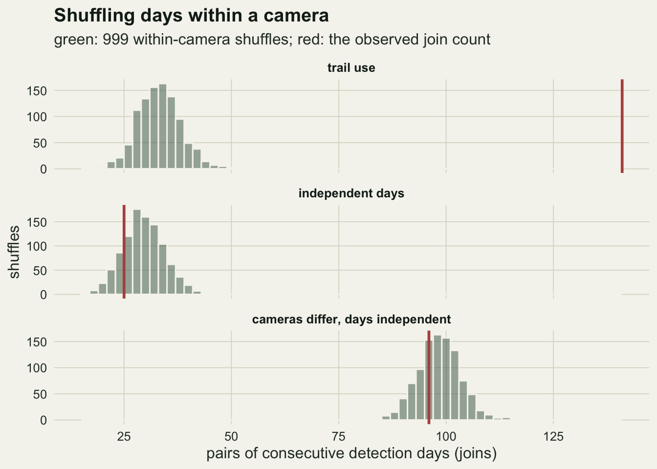
What to report
State the occasion length and why it was chosen, and report the join count check (observed joins, the shuffled mean, the permutation p) on the daily detection matrix before any collapsing, with the daily-total check from the same shuffles beside it. If the join count check is clean, daily occasions are defensible as far as day-to-day dependence goes, and they keep day-level detection covariates available. A clean result is weaker evidence than it looks: the test’s power depends on the number of detected cameras and on the strength of the memory, so a smaller survey can miss a chain like the weaker one here, which the test caught in 100.0 per cent of surveys of this size but which still pulled the daily estimate to 0.477 with coverage 92.0 per cent.
If the join count check flags dependence, look at the daily-total check before abandoning daily occasions. When it fires as well, detection that varies from day to day at every camera together can produce the joins on its own; on the shared-weather surveys here the daily estimate was close to the truth with near-nominal coverage, so that flag calls for a look at the day-level variables (a weather record, a lure refresh) in the detection model rather than for wider occasions, although it does not rule out memory as well. When only the join count fires, do not report a daily-occasion occupancy estimate on its own. On this design the estimate at daily occasions was 0.405 for a truth of 0.5, with intervals that covered in 36.2 per cent of surveys. Either fit a model with the dependence in it, or widen the occasions and say what that cost. Reporting the estimate at two or three occasion lengths side by side is cheap and shows the reader whether it is still moving; here it moved from 0.405 to 0.486 across the six lengths.
Do not present the longest occasion as the correct one. At fifteen days the estimate was still 0.014 short and the coverage 94.2 per cent, and any day-level detection covariate was reduced to a window mean. With five-day occasions the covariate was found in 89.0 per cent of surveys and with fifteen-day occasions in 22.5 per cent. The occasion length is a compromise between those two costs, and the numbers for both belong in the methods.
Honest limits
The chain simulated here is the simplest possible memory: one day back, the same for every camera, with the detections themselves carrying the dependence. Real trail use has longer memory (a territory holder that shifts its route for a week) and camera-level differences at the same time, and the heterogeneous surveys above show that the second problem biases occupancy even without the first. The dependent model fitted in this post is the fully observed, trap-response form; the version with a hidden local-presence state and imperfect detection on top of it, the other form in Hines and colleagues 2010, was not implemented or tested here. Their own simulations are a warning about that gap: with dependence in local presence, they report that the bias was smaller than the standard model’s for the trap-response model and negligible only for the spatial process model, so the trap-response fit that works here because it is the true model reduces but does not remove the bias when the memory sits in the animal’s presence rather than in the detections.
Everything is one design: 150 cameras, occupancy one half, thirty days, and a daily rate near a tenth. The Goldstein 2024 summary reports strong bias when surveys are short and detection rates are low; the direction of that statement was not tested here, since both the survey length and the daily rate were fixed. The weaker chain gave a smaller bias, which is the only sensitivity this post measured.
The coverage figures are for the Wald interval on the logit scale. A profile likelihood interval might behave differently at few occasions, and nothing here measures it.
The join count test was run as a within-camera permutation of the daily matrix. That is one way to build the reference distribution; the test in the literature that Goldstein and colleagues recommend was not checked against this implementation line by line, and anyone applying their recommendation should follow the published definition rather than this one. The join count test also fires on detection that varies from day to day at every camera together. The daily-total check separates that from memory when only one of them is present; a survey with both would fire both checks, no such mixed survey was simulated, and nothing here separates the two. The permutation also assumes every camera ran for all thirty days. Missing days break the shuffle, and a camera that failed for a week needs the shuffle restricted to the days it ran.
References
Goldstein BR, Jensen AJ, Kays R, Cove MV, McShea WJ, Rooney B, Kierepka EM, Pacifici K 2024 Methods in Ecology and Evolution 15(7):1177-1191 (10.1111/2041-210X.14359)
Hines JE, Nichols JD, Royle JA, MacKenzie DI, Gopalaswamy AM, Kumar NS, Karanth KU 2010 Ecological Applications 20(5):1456-1466 (10.1890/09-0321.1)